Guided Tutorial Extras Sample Rates
NOTE: This tutorial has been deprecated in GR 3.8.
E1.1. Adjusting the Sample Rate in GRC
We start with the same flowgraph introduced in Section 2.3.1:

This flowgraph generates a sine wave and plots it in time and frequency along with a slider that allows us to dynamically adjust the sample rate while we hold the frequency of the sine wave constant.
The output looks like:
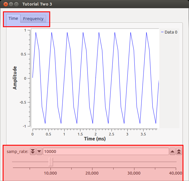
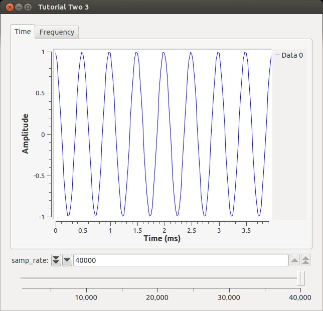
Our signal of the sine wave looks pretty bad with all those straight lines! What we can do is change the samp_rate variable without having to re-generate the flowgraph. Let's increase the samp_rate to the maximum by sliding the slider to full right. What should the output appear as?
{{collapse(View Output...)
 }}
}}
E1.2. Testing the Nyquist Frequency
Now let's turn to the Frequency tab.
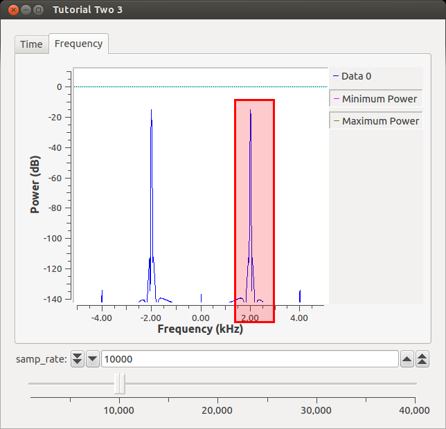
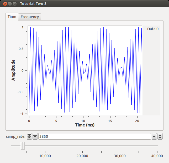
At a sampling rate of 10k, we are able to reproduce our original frequency (2 kHz). If we sample higher, we will still get a peak at 2 kHz. Nyquist tells us that once we sample at anything lower than 2*original_signal_freq, we will be unable to reproduce the signal. We read that in a textbook, though, so we are not convinced. Let's slide our samp_rate to 3.85 kHz. What happens to the Time waveform?
{{collapse(View Output...)
 }}
}}
Well, it definitely doesn't look like a sine wave anymore, but our eyes can be deceived so let's turn to the FFT to get its frequency.
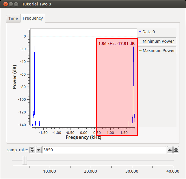
We see that the frequency is no longer at 2 kHz like it should be based on our input signal. Instead, since we are 0.15 kHz below the Nyquist rate, the signal has "folded-over" and is now 0.15 kHz below its actual frequency (my cursor was a little off :( ). This is simple sanity check that GNU Radio simulates DSP theory.
For a more detailed explanation of sample rate and for the FFT
E2.3. A Note on Resampling
Now that we know about Nyquist and how things go bad if we aren't paying attention to rates, we can talk about resampling. Resampling is used to change the sampling rate of a signal in order to meet the requirements of another system such as the sampling rate of a sound card. There are two important terms: interpolation and decimation. Interpolation adds samples, decimation removes samples. So let's understand what that means with an example:
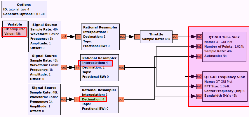
Semi-Detailed Changes:
- samp_rate to 48e3
- Interpolation to 4
- Decimation to 4
- Number of Inputs to 3 (on both sinks)
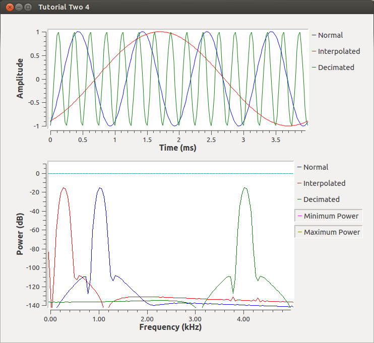
By default the line colors are in0-blue, in1-red, in2-green however the colors and other options such as line width or labels can easily be changed in the config tab on any of the qt instrumentation sinks. Can we guess what will happen for both time and frequency to the Interpolated signal? The Decimated signal?
{{collapse(Resampling)
 }}
}}
We can see that resampling changes the sampling rate of our original signal by the resampling/decimation/interpolation factor. We then use the scaled sampling rate on a non-scaled sampling rate (our sinks) therefore the sinks appear to receive frequencies that are higher/lower than the original signal. This becomes important when we we make blocks that will interface with hardware or modulators/demodulators that require a certain sample rate to work efficiently. We will explore one such example later. For now it is important for us to remember that sampling rates should match between our blocks or we will receive frequency scaling.
An important note about the above flowgraph. While we were able to run this and draw the results, this flowgraph will stop and hang unexpectedly. The QT sinks are not built to allow us to plot data being received at different sample rates between the different inputs. It is best here to plot each sample rate domain in a different GUI sink, instead. Here, we use it to easily show the comparisons between the three sampling rates.