Polyphase Clock Sync
Timing synchronizer using polyphase filterbanks.
This block performs timing synchronization by minimizing the derivative of the filtered signal, which in turn maximizes the SNR and minimizes ISI (Inter-Symbol Interference).
Details of the Polyphase Clock Sync Block
There are various algorithms that we can use to recover the clock at the receiver, and almost all of them involve some kind of feedback control loop. Those that don't are generally data aided using a known word like a preamble. This block does three things for us. First, it performs the clock recovery. Second, it does the receiver matched filter to remove the ISI. Third, it down-samples the signal.
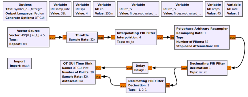
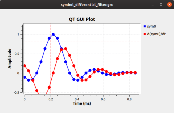
The block works by calculating the first differential of the incoming signal, which will be related to its clock offset. If we simulate this very simply at first, we can see how the differential filter will work for us. First, using the example flowgraph symbol_differential_filter.grc, we can see how everything looks perfect when our rate parameter is 1 (i.e., there is no clock offset). The sample we want is obviously at 0.22 ms. The difference filter ([-1, 0, 1]) generates the differential of the symbol, and as the following figure shows, the output of this filter at the correct sampling point is 0. We can then invert that statement and instead say when the output of the differential filter is 0 we have found the optimal sampling point.
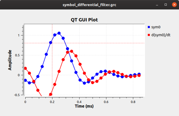
What happens when we have a timing offset? That output is shown below shows that the timing offset where the peak of the symbol is off and the derivative filter does not show us a point at zero.
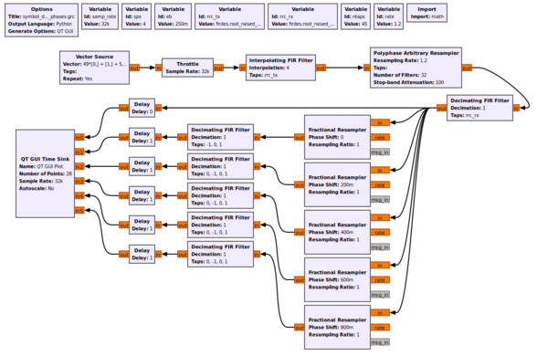
Instead of using a single filter, what we can do is build up a series of filters, each with a different phase. If we have enough filters at different phases, one of them is the correct filter phase that will give us the timing value we desire. Let's look at a simulation that builds 5 filters, which means 5 different phases. Think of each filter as segmenting the unit circle (0 to 2pi) into 5 equal slices. Using the example flowgraph symbol_differential_filter_phases.grc, we can see how this helps us. Notice here that we are using the fractional resampler here because it makes it easy to do the phase shift (between 0 and 1), but it also changes the filter delays of the signals, so we correct for that using the follow-on delay blocks.
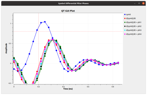
The figure below now gives us an idea of what we're dealing with, although it's a bit inexact. What we can see is that the signal labeled as d(sym0)/dt + phi3 has a sample point at 0. This tells us that our ideal sampling point occurs at this phase offset. Therefore, if we take the RRC filter of our receiver and adjust its phase by phi3 (which is 3*2pi/5), then we can correct for the timing mismatch and select the ideal sampling point at this sample time.
But as we have discussed, this is only a simulated approximation; in reality, the samples of each filter wouldn't occur at the same point in time. We have to up-sample by the number of filter (e.g., 5) to really see this behavior. However, that can clue us into what's happening a bit farther. We can look at these different filters as parts of one big filter that is over-sampled by M, where M=5 in our simple example here. We could up-sample our incoming signal by this much and select the point in time where we get the 0 output of the difference filter. The trouble with that is we are talking about a large amount of added computational complexity, since that is proportional to our sample rate. Instead, we're working on filters of different phases at the incoming sample rate, but with the bank of them at these different phases, we can get the effect of working with the over-sampled filter without the added computational cost.
So in our example above, we offset our sampling rate by some known factor of 1.2 and found that we could use one of five filters as the ideal sampling point. Unfortunately, we really only have 5 different phases we can exactly produce and correct for here. Any sampling offset between these phases will still produce a mistimed sample with added ISI. So instead, we use way more than 5 filters in our clock recovery algorithm. Without exploring the math (see harris' book referenced above), we can use 32 filters to give us a maximum ISI noise factor that is less than the quantization noise of a 16 bit value. If we want more than 16 bits of precision, we can use more filters.
So what? We have a large bank of filters where one of them is at (or very close to) the ideal sampling phase offset. How do we automatically find that? Well, we use a 2nd order control loop. The error signal for the recovery is the output of the differential filter. The control loop starts at one of the filters and calculates the output as the error signal. It then moves its way up or down the bank of filters proportionally to the error signal, and so we're trying to find where that error signal is closest to 0. This is our optimal filter for the sampling point. And because we expect the transmit and receive clocks to drift relative to each other, we use a second order control loop to acquire both the correct filter phase as well as the rate difference between the two clocks.
GNU Radio comes with an example found in the digital examples directory called example_timing.py. You can run this script on your own to see the convergence behavior of the Polyphase Clock Sync block.
This block also can use the 'time_est' tag which is generated by a Correlation Estimator block. That helps to correct symbol timing offset.
Reference
f. j. harris and M. Rice, "Multirate Digital Filters for Symbol Timing Synchronization in Software Defined Radios", IEEE Selected Areas in Communications, Vol. 19, No. 12, Dec., 2001. [1]
Parameters
(R): Run-time adjustable
- Samples/Symbol
- The clock sync block needs to know the number of samples per symbol, because it defaults to return a single point representing the symbol. The sps can be any positive real number and does not need to be an integer.
- Loop Bandwidth (R)
- The loop bandwidth is used to set the gain of the inner control loop (see: [2]).
- This should be set small (a value of around 2pi/100 is suggested in that blog post as the step size for the number of radians around the unit circle to move relative to the error).
- Taps (R)
- One of the most important parameters for this block is the taps of the filter.
- One of the benefits of this algorithm is that you can put the matched filter in here as the taps, so you get both the matched filter and sample timing correction in one go. So create your normal matched filter. For a typical digital modulation, this is a root raised cosine filter.
- The number of taps of this filter is based on how long you expect the channel to be; that is, how many symbols do you want to combine to get the current symbols energy back (there's probably a better way of stating that). It's usually 5 to 10 or so. That gives you your filter, but now we need to think about it as a filter with different phase profiles in each filter. So take this number of taps and multiply it by the number of filters. This is the number you would use to create your prototype filter. When you use this in the PFB filerbank, it segments these taps into the filterbanks in such a way that each bank now represents the filter at different phases, equally spaced at 2pi/N, where N is the number of filters.
- Filter Size
- The number of filters can also be set and defaults to 32. With 32 filters, you get a good enough resolution in the phase to produce very small, almost unnoticeable, ISI. Going to 64 filters can reduce this more, but after that there is very little gain for the extra complexity.
- Initial Phase
- The initial phase is another settable parameter and refers to the filter path the algorithm initially looks at (i.e., d_k starts at init_phase). This value defaults to zero, but it might be useful to start at a different phase offset, such as the mid-point of the filters.
- Maximum Rate Deviation
- The next parameter is the max_rate_devitation, which defaults to 1.5. This is how far we allow d_rate to swing, positive or negative, from 0. Constraining the rate can help keep the algorithm from walking too far away to lock during times when there is no signal.
- Output SPS
- The osps is the number of output samples per symbol. By default, the algorithm produces 1 sample per symbol, sampled at the exact sample value. This osps value was added to better work with equalizers, which do a better job of modelling the channel if they have 2 samps/sym.
Example Flowgraph
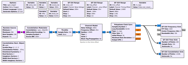
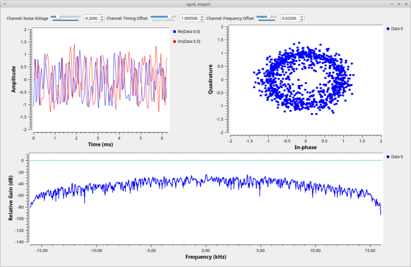
This flowgraph is taken from the QPSK_Mod_and_Demod tutorial.
Source Files
- C++ files
- Complex input
- Float input
- Header files
- Complex input
- Float input
- Public header files
- Complex input
- Float input
- Block definition
- [3]
