GR-ATA Tutorial: Difference between revisions
EllieWhite (talk | contribs) No edit summary |
EllieWhite (talk | contribs) No edit summary |
||
| (7 intermediate revisions by the same user not shown) | |||
| Line 10: | Line 10: | ||
Before beginning this tutorial, please make sure that you have installed GNU Radio version 3.8, gr-ata, and the ATA-Utils library, following the instructions here: [https://wiki.gnuradio.org/index.php/GNURadio@theATA#Setting_up_the_software Setting up the software] | Before beginning this tutorial, please make sure that you have installed GNU Radio version 3.8, gr-ata, and the ATA-Utils library, following the instructions here: [https://wiki.gnuradio.org/index.php/GNURadio@theATA#Setting_up_the_software Setting up the software] | ||
=== Warnings === | |||
When observing with the ATA, please be cautious in your choice of sources -- while natural sources and satellites with weaker signals are generally fine to observe with the ATA, observing a strong satellite could cause expensive damage to the antenna's electronics. If you are wanting to do a capture of a satellite or strong source (like the Sun) but are unsure of the safety of it, '''please inform ATA staff and get their permission and feedback''' before moving ahead. | |||
== Tutorial 1: A Simulated ATA Observation == | == Tutorial 1: A Simulated ATA Observation == | ||
| Line 61: | Line 65: | ||
== Tutorial 2: Observing with the ATA == | == Tutorial 2: Observing with the ATA == | ||
Although in many ways performing a real observation with the ATA is similar to the simulated observation described above, there are some subtle differences that are worth noting, and which I will describe in this tutorial. | Although in many ways performing a real observation with the ATA is similar to the simulated observation described above, there are some subtle differences that are worth noting, and which I will describe in this tutorial. '''Recommended:''' if you'd like to watch the ATA antennas move as you're carrying out your observation, check out this webcam which you can access if you're connected via the ATA VPN server: http://cam3cntl.hcro.org/. | ||
My preferred way of running an observation is to run a flowgraph for antenna control and a separate flowgraph for data collection (see Tutorial 3 for a data collection guide), which I start after the antenna has landed on its source. It is possible to run the control blocks and the data acquisition blocks in the same flowgraph -- I don't recommend this, however, as you will be collecting a lot of garbage data at the beginning of your observation while the antenna is slewing to the correct source. | |||
=== Reserving and Releasing the Array === | |||
Before you run any flowgraphs, if you have received time on the Allen Array and wish to conduct an observation, you must run a script to claim the array. In the [https://github.com/SETIatHCRO/gr-ata/tree/master/examples examples] folder, you should find two scripts, ata-set-alarm.py and ata-unset-alarm.py. | |||
Before you start observing, run the following command with your username and message in place of the placeholders: | |||
'''python3 ata-set-alarm.py -u username -m 'message describing what you're doing with the array' ''' | |||
After you have completed your observation session, you must release the array for others to use. In this case you should run the following command: | |||
'''python3 ata-unset-alarm.py -u username -m 'exit message' ''' | |||
Keep these steps in mind whenever you observe with the ATA. | |||
=== Track Scan Observation === | === Track Scan Observation === | ||
| Line 69: | Line 90: | ||
[[File:Offline-tutorial-img1.png|800px]] | [[File:Offline-tutorial-img1.png|800px]] | ||
You will need to update the properties of the Control block. In the '''Username''' space, type in the username you were assigned when you were given an account on the ATA computer, and make sure you have selected '''Observing Mode'''. The purpose of entering your username here is to check what permissions you have on the array. If you have spoken with ATA staff and have explicit permission to change the entire array's operating frequency (there is only 1 LO so even if you think you are changing the frequency for just your antennas, without a safety check you could change the frequency of the entire array and disrupt another observer's session), and have subsequently locked out the array under your username, the flowgraph will be able to change the LO center frequency. However, if you are not the primary user and have not locked out the array, the flowgraph will not allow you to | You will need to update the properties of the Control block. In the '''Username''' space, type in the username you were assigned when you were given an account on the ATA computer, and make sure you have selected '''Observing Mode'''. The purpose of entering your username here is to check what permissions you have on the array. If you have spoken with ATA staff and have explicit permission to change the entire array's operating frequency (there is only 1 LO so even if you think you are changing the frequency for just your antennas, without a safety check you could change the frequency of the entire array and disrupt another observer's session), and have subsequently locked out the array under your username, the flowgraph will be able to change the LO center frequency. However, if you are not the primary user and have not locked out the array, the flowgraph will not allow you to run in Observing Mode. | ||
[[File:Obsmode-tutorial1.png|500px]] | [[File:Obsmode-tutorial1.png|500px]] | ||
| Line 75: | Line 96: | ||
As before, now open the '''Track Scan''' block's properties. This time, for the Frequency, you must enter a value between 1000 MHz and 15000 MHz, as these are the lower and upper bounds of the array's operating frequencies. Note that the observing band is xx MHz wide, and this band will be centered on whatever frequency you indicate in the box (again, if you have LO permissions -- if not you'll just be tuning your antenna to that center frequency). In the case where you do '''not''' have LO permissions, it is a good idea to check what the center frequency of the array is set to and pick your center frequency somewhere within the current observing band. | As before, now open the '''Track Scan''' block's properties. This time, for the Frequency, you must enter a value between 1000 MHz and 15000 MHz, as these are the lower and upper bounds of the array's operating frequencies. Note that the observing band is xx MHz wide, and this band will be centered on whatever frequency you indicate in the box (again, if you have LO permissions -- if not you'll just be tuning your antenna to that center frequency). In the case where you do '''not''' have LO permissions, it is a good idea to check what the center frequency of the array is set to and pick your center frequency somewhere within the current observing band. | ||
For the antennas list, make sure to select antennas from the following list: '''1a, 1b, 1c, 1d, 1e, 1f, 1g, 1h, 1j, 1k, 2a, 2b, 2c, 2d, 2e, 2f, 2g, 2h, 2j, 2k, 2l, 2m, 3c, 3d, 3e, 3f, 3g, 3h, 3j, 3l, 4e, 4f, 4g, 4h, 4j, 4k, 4l, 5b, 5c, 5e, 5g, 5h'''. Note that only | For the antennas list, make sure to select antennas from the following list: '''1a, 1b, 1c, 1d, 1e, 1f, 1g, 1h, 1j, 1k, 2a, 2b, 2c, 2d, 2e, 2f, 2g, 2h, 2j, 2k, 2l, 2m, 3c, 3d, 3e, 3f, 3g, 3h, 3j, 3l, 4e, 4f, 4g, 4h, 4j, 4k, 4l, 5b, 5c, 5e, 5g, 5h'''. Note that only antennas '''1a, 1c, 1f, 2a, 2b, 2h, 3c, 1k, 4g, and 5c''' are capable of acquiring data via a USRP at this moment; the other antennas are in the process of being refurbished. | ||
Coordinate type is the same as before -- you can choose Catalog Identifier, RA / Dec, or Az / El. In Offline Mode it really doesn't matter what source ID you enter if you select Catalog Identifier, but in '''Observing Mode''' you must put in an identifier from the [https://github.com/SETIatHCRO/gr-ata/blob/master/docs/ata-catalog.txt catalog], if you put in an unknown source the program will throw an error. RA / Dec and Az / El fields must be numbers. When the observation begins, the software will check if your source location of interest is above the horizon; if not it will tell you so and will not attempt to observe your source. | Coordinate type is the same as before -- you can choose Catalog Identifier, RA / Dec, or Az / El. In Offline Mode it really doesn't matter what source ID you enter if you select Catalog Identifier, but in '''Observing Mode''' you must put in an identifier from the [https://github.com/SETIatHCRO/gr-ata/blob/master/docs/ata-catalog.txt catalog], if you put in an unknown source the program will throw an error. RA / Dec and Az / El fields must be numbers. When the observation begins, the software will check if your source location of interest is above the horizon; if not it will tell you so and will not attempt to observe your source. | ||
| Line 81: | Line 102: | ||
[[File:Obsmode-tutorial2.png|500px]] | [[File:Obsmode-tutorial2.png|500px]] | ||
Now, | Now, before running your flowgraph, add one more block -- an '''IF switch block.''' In the switch 1 and / or switch 2 drop-down list, select which antenna(s) you'd like to observe with (this will configure the IF Switch so that your USRPs will take in data from the correct antennas). | ||
If you now run your flowgraph, you should see various messages printed in the terminal window indicating the progress of your observation. This may take awhile depending on the speed of your connection to the ATA machine so be patient, practice meditation, pet your dog / cat / iguana, etc. for a bit while you wait. | |||
The antenna(s) will track on the source until you stop the flowgraph. | |||
=== Changing the target source during an observing run === | === Changing the target source during an observing run === | ||
| Line 95: | Line 118: | ||
Then run the flowgraph again. Now, the QT GUI message edit box should show up; to slew to a new source, type '''source_id''' in the left-hand box and the name of the source you want to slew to (again, it must be from the catalog linked in the last section) in the right-hand box, then hit the '''Enter''' key and after a bit the antennas should start slewing to the new target. Alternatively, if you'd like to enter an RA / Dec or Az / El pair in the message box, type "radec" in the left-hand box and then your right ascension, declination pair separated by a comma in the right-hand box (like: ra,dec). Similarly, for Az / El, you can type "azel" in the left-hand box, then the coordinate pair (like: az,el) in the right-hand box. Recall the prior warning that if you type non-number symbols in the right-hand box when trying to slew to a target given by an RA / Dec or Az / El pair, it will print an error message. | Then run the flowgraph again. Now, the QT GUI message edit box should show up; to slew to a new source, type '''source_id''' in the left-hand box and the name of the source you want to slew to (again, it must be from the catalog linked in the last section) in the right-hand box, then hit the '''Enter''' key and after a bit the antennas should start slewing to the new target. Alternatively, if you'd like to enter an RA / Dec or Az / El pair in the message box, type "radec" in the left-hand box and then your right ascension, declination pair separated by a comma in the right-hand box (like: ra,dec). Similarly, for Az / El, you can type "azel" in the left-hand box, then the coordinate pair (like: az,el) in the right-hand box. Recall the prior warning that if you type non-number symbols in the right-hand box when trying to slew to a target given by an RA / Dec or Az / El pair, it will print an error message. | ||
=== On-Off Observation === | |||
As was true for the simulated observation, if you'd like to use the On-Off block instead of the Track Scan block, almost all of the instructions for the Track Scan observation are equally applicable. Set up the flowgraph like this: | |||
[[File:Obsmode-tutorial5.png|800px]] | |||
For the On-Off block, in addition to setting the center frequency, antennas list, and source location as you did before, for the On-Off block you will also need to indicate your on-source duration and the amount of offsets which you wish for the antenna to slew away from the source for the off-source part of the observation. Add an '''IF Switch block''' with the proper antennas selected as before. | |||
[[File:Obsmode-tutorial4.png|500px]] | |||
When you play this flowgraph, the antenna(s) will first slew onto your target source, and will track on that source for the given duration, then slew off-source by the offset amount you indicated in the block's properties. The antenna(s) will stay on the offset source until you stop the flowgraph. | |||
== Tutorial 3: Data Collection == | |||
As mentioned above, once you have pointed your antenna(s) at a target source you can run a flowgraph to record data. There are two ways to do this -- one is to record the complex voltages straight from the USRP source block, which produces very large files but saves the phase information from the data; and the other is to do some DSP to the signal before recording if you are not concerned about preserving the phase information of the signal and would prefer to have a smaller filesize. In the first section below we're going to go over the first method. | |||
=== Saving Raw Voltage Data === | |||
For this tutorial, please open the record_raw_data.grc example from the gr-ata [https://github.com/SETIatHCRO/gr-ata/tree/master/examples examples] folder in the GNU Radio companion. This example shows you how to record one polarization of data from a single antenna. The antenna you will be receiving data from will have been set by the antenna you selected in the IF Switch block when you ran the control flowgraph to point your antennas. | |||
[[File:Record-raw-data.png|800px]] | |||
Before running the flowgraph, please make sure: | |||
* You have set the right sampling rate in the '''samp_rate''' variable box. The USRPs can go up to 200 MS/s, or that number divided by any integer. The sample rate determines your bandwidth so be mindful of that (and also file size) when setting your sample rate. | |||
* Make sure the center frequency in the '''fc''' variable box is set to 629 MHz; this ensures your USRP is recorded data centered on the LO frequency you indicated when you ran your flowgraph to initialize and point the antennas previously. | |||
* Make sure '''src_name''' is set to the right identifier for your source. This doesn't affect your data, it just ensures you have a descriptive filename. | |||
In the USRP source block, check that: | |||
* The Device Address is set to "serial=31D3A48" to use the Ettus N321 | |||
* Mb0 Clock Source is set to internal | |||
* Mb0 Subdev Spec is empty | |||
* In RF Options, Antenna 0 is set to TX/RX | |||
Note that the complex conjugate block in this flowgraph corrects for the fact that the raw voltages are flipped coming in to the system. | |||
Now you can run the flowgraph! Note that if you start seeing OO's appear in the output you should stop recording and try reducing the sampling rate because in that case it is likely that you are saving data more quickly than the system can handle it. | |||
If you are recording data successfully and not seeing OO's, just record for as long as you like and then click the Stop sign when you are finished. | |||
It should not be too difficult to extend this example flowgraph to accept input from multiple channels and / or multiple USRPs. | |||
=== Saving spectrum data === | |||
For this tutorial, please open the record_psd_data.grc flowgraph from the [https://github.com/SETIatHCRO/gr-ata/tree/master/examples examples] folder in GNU Radio companion. Setup for this type of data recording is, in many ways, similar to the initialization for recording raw data but there are a few additions. | |||
As for the raw recording, make sure that in the USRP source block: | |||
* The Device Address is set to "serial=31D3A48" to use the Ettus N321 | |||
* Mb0 Clock Source is set to internal | |||
* Mb0 Subdev Spec is empty | |||
* In RF Options, Antenna 0 is set to TX/RX | |||
And also check that: | |||
* You have set the right sampling rate in the '''samp_rate''' variable box. The USRPs can go up to 200 MS/s, or that number divided by any integer. The sample rate determines your bandwidth so be mindful of that (and also file size) when setting your sample rate. | |||
* Make sure the center frequency in the '''fc''' variable box is set to 629 MHz; this ensures your USRP is recorded data centered on the LO frequency you indicated when you ran your flowgraph to initialize and point the antennas previously. | |||
* Make sure '''src_name''' is set to the right identifier for your source. This doesn't affect your data, it just ensures you have a descriptive filename. | |||
* Set the '''decimation''' variable to the number of vectors you want to integrate over. Higher decimation = better signal to noise and smaller filesize, but also lower time resolution in your resulting data. | |||
* Set the '''fftsize''' variable to the number of points you want your FFT to be -- note it should be a power of 2. Note that the larger the fftsize, the better the spectral resolution but the lower the time resolution. | |||
[[File:Record-psd-data.png|800px]] | |||
Once you are certain everything is set up properly, go ahead and run the flowgraph, and remember to turn it off when you are finished or you will accrue lots of data. | |||
== Tutorial 4: Playing back recorded data == | |||
Since I've posted tutorials on how to record both raw and spectrum data, I'd like to now cover how to play back the data you've recorded and do some analysis on it. This tutorial will be split into two sections like Tutorial 3 as you will need to plot raw and spectrum data differently. Below is a sample plot showing an example of what the resulting plots from both methods will look like: | |||
[[File:l-band-plot.png|800px]] | |||
Note that the provided flowgraphs not only plot the results against frequency, but they also have the capability to plot the results converted to a velocity with respect to local standard of rest (V_LSR) if you have a need for it. | |||
=== Plotting a spectrum from a raw data file === | |||
To plot a spectrum from a raw data file, you will need to do a bit of extra processing to get the raw data from voltage to power spectrum form; these processing steps are done by the blocks between the file source block and the vector sink block as shown below; this flowgraph can be found in [https://github.com/SETIatHCRO/gr-ata/tree/master/examples examples] under the name plot_from_raw.grc. | |||
[[File:Plot-from-raw.png|800px]] | |||
Of course the first step is to make sure you've selected the proper data file in the file sink block. | |||
To process the data to your liking, make sure you have: | |||
* Set the '''fftsize''' variable to the number of points you want your FFT to be -- note it should be a power of 2. Note that the larger the fftsize, the better the spectral resolution but the lower the time resolution. | |||
* Set the '''decimation''' variable to the number of vectors you want to integrate over. Higher decimation = better signal to noise and smaller filesize, but also lower time resolution in your resulting data. | |||
For the spectrum plot, it is important to make sure that you have: | |||
* Set the '''cfreq''' equal to the value that your LO was set to during your observation (1420 MHz in this case). | |||
* Set the '''samp_rate''' equal to the value of the sample rate used during recording | |||
If you don't want to plot VLSR, just disable or delete that block. If you do, however, you must make sure to: | |||
* Set the '''rest_freq''' to the rest frequency of the spectral line you want to observe. | |||
* Open the variable '''v_corr''', and in the function call (ie v.vlsr_correction('2010-03-26T15:16:33', 2.451075, 61.873500)) make sure the first field is a timestamp of the beginning of the observation in the same format as shown here (the filenames are automatically saved with the timestamp in their title); the second field is right ascension in hour angle and the third field is declination in decimal degrees. | |||
At this point, if you have ensured everything is to your liking, you should be good to go to run the flowgraph and plot your data! | |||
=== Plotting a spectrum from a pre-processed data file === | |||
If you want to plot a spectrum from a data file which is already processed and saved in power spectrum format, the process is simpler. For this tutorial use the plot_from_psd.grc flowgraph found in [https://github.com/SETIatHCRO/gr-ata/tree/master/examples examples]. | |||
Just make sure to: | |||
* Enter the proper filepath in the File Sink block. | |||
* Set the '''cfreq''' equal to the value that your LO was set to during your observation (1420 MHz in this case). | |||
* Set the '''samp_rate''' equal to the value of the sample rate used during recording divided by two (since the samples are real, not complex). | |||
Again, if you don't want to plot VLSR, just disable or delete that block. If you do, however, you must make sure to: | |||
* Set the '''rest_freq''' to the rest frequency of the spectral line you want to observe. | |||
* Open the variable '''v_corr''', and in the function call (ie v.vlsr_correction('2010-03-26T15:16:33', 2.451075, 61.873500)) make sure the first field is a timestamp of the beginning of the observation in the same format as shown here (the filenames are automatically saved with the timestamp in their title); the second field is right ascension in hour angle and the third field is declination in decimal degrees. | |||
Press play and you should be good to go! | |||
[[File:Plot-from-psd.png|800px]] | |||
Latest revision as of 23:42, 14 August 2020
On this page we'll walk through a few scenarios of running observations (both real and simulated) on the Allen Telescope Array with GNU Radio and the gr-ata module.
Step 0: Before you start...
In order to run an observation on the ATA, please know that you must coordinate with ATA staff to avoid interfering with science observing campaigns onsite.
Please find a catalog of astronomical sources recognized by the gr-ata module here: https://github.com/SETIatHCRO/gr-ata/blob/master/docs/ata-catalog.txt
Before beginning this tutorial, please make sure that you have installed GNU Radio version 3.8, gr-ata, and the ATA-Utils library, following the instructions here: Setting up the software
Warnings
When observing with the ATA, please be cautious in your choice of sources -- while natural sources and satellites with weaker signals are generally fine to observe with the ATA, observing a strong satellite could cause expensive damage to the antenna's electronics. If you are wanting to do a capture of a satellite or strong source (like the Sun) but are unsure of the safety of it, please inform ATA staff and get their permission and feedback before moving ahead.
Tutorial 1: A Simulated ATA Observation
In this first tutorial, we will run through a simulated offline "observing" session -- although in this tutorial we won't be conducting real observations, it is a good idea to start here to make sure you understand what the gr-ata blocks are doing and get familiar with the system and terminology before starting your real observation. This mode of running the gr-ata blocks does not require you to be able to connect to the ATA computers, either, so it is a good place to start.
Simulated Track Scan observation
Let's first try a very simple test. Drag and drop an ATA Track Scan block and an ATA Control block into an empty flowgraph and connect their message ports as shown below.
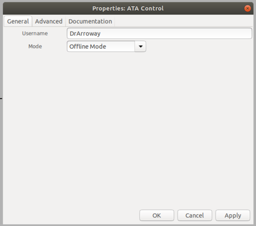
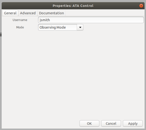
Make sure you have changed the ID field in the automatically-populated Options block to something besides default or the program won't run. Now double click the Control block to bring up the Properties window. Enter your username (for the offline tutorial this field doesn't matter, just type anything), then select Offline Mode from the Mode drop-down list, as shown. Click OK to apply your changes and close the Properties window.
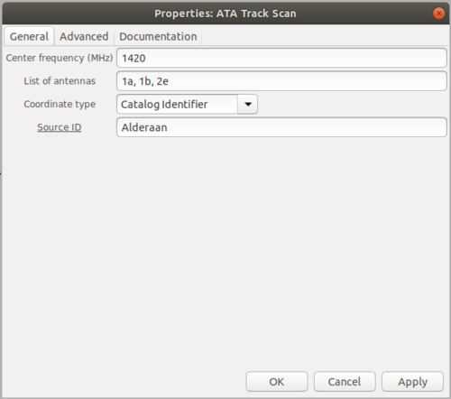
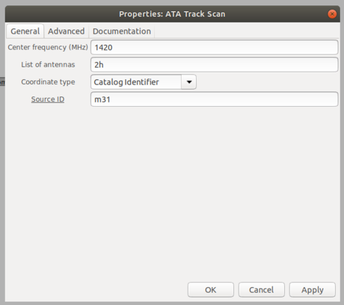
Now double click on the Track Scan block to view its properties. The first field is Frequency (MHz) -- enter any number of your choice here (it doesn't really matter what you enter in Offline Mode, just so long as it is a number). The next field is List of antennas; this field requires a string or list of strings as input, entered as shown. To simulate a real observing session, you could enter one or more of the actual antenna names of ATA antennas by choosing from the following list: 1a, 1b, 1c, 1d, 1e, 1f, 1g, 1h, 1j, 1k, 2a, 2b, 2c, 2d, 2e, 2f, 2g, 2h, 2j, 2k, 2l, 2m, 3c, 3d, 3e, 3f, 3g, 3h, 3j, 3l, 4e, 4f, 4g, 4h, 4j, 4k, 4l, 5b, 5c, 5e, 5g, 5h as shown. Next, select how you want to enter your target source in the Coordinate Type drop-down -- you can choose Catalog Identifier (as in the example below), RA / Dec, or Az / El. If you choose Catalog Identifier, a Source ID field will be displayed, where you can enter a source name -- in Offline Mode this source name can be anything, but in Observing Mode you must select an identifier from this catalog. If you select RA / Dec, separate RA and Dec fields will be displayed where you can enter your coordinates in decimal degrees; similarly if you select Az / El, Az and El fields will be displayed as well.
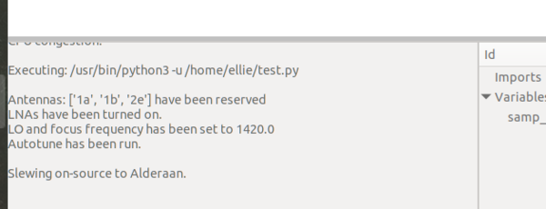
Now that you have connected the two blocks and filled out the required fields, you can save your flowgraph then hit Run. You should see output in the terminal window as shown:
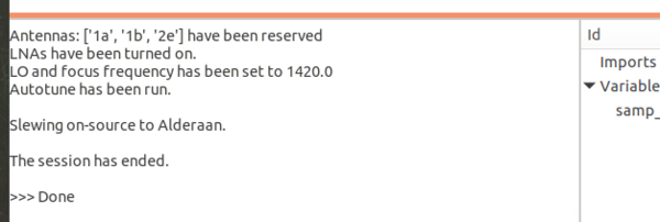
Once the text has printed, you can stop the flowgraph, and an exit message will be printed:
Changing the target source during a simulated observation
Another thing you can do is test out the real-time message passing capability of the Track Scan block. First, drag and drop a QT GUI Message Edit Box and connect it to the Track Scan block's msg_in port as shown:
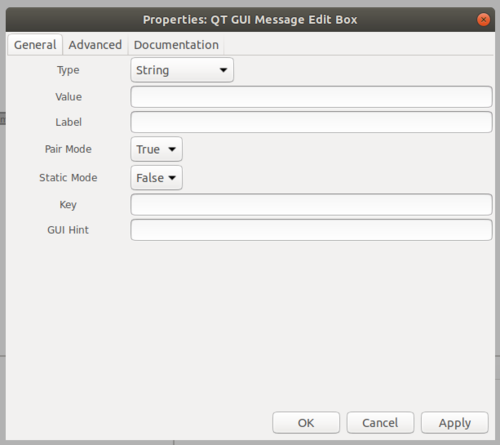
Edit the Properties of the Message Edit box so they match what's shown below:
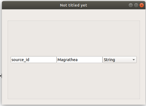
Then run the flowgraph again. Now, the QT GUI message edit box should show up as in the image below; to slew to a new source, simply type source_id in the left-hand box and the name of the source you want to slew to in the right-hand box, then hit the Enter key and the text in the GNU Radio terminal window should update to say slewing on-source to {source name}. Alternatively, if you'd like to enter an RA / Dec or Az / El pair in the message box, type "radec" in the left-hand box and then your right ascension, declination pair separated by a comma in the right-hand box (like: ra,dec). Similarly, for Az / El, you can type "azel" in the left-hand box, then the coordinate pair (like: az,el) in the right-hand box. If you type non-number symbols in the right-hand box when trying to slew to a target given by an RA / Dec or Az / El pair, it will print an error message, so just be mindful of that.
Simulated On-Off observation
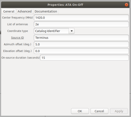
If you wish to use the On-Off block instead of the Track Scan block, almost all of the instructions above are equally applicable. However, in addition to setting the center frequency, antennas list, and source location as you did in the Track Scan block, you will also need to indicate your on-source duration and the amount of offsets which you wish for the antenna to slew away from the source for the off-source part of the observation:
When you play the flowgraph with the On-Off block in place of the Track Scan block, a message will be printed that says the (imaginary) antennas have "slewed" on source, then after the given duration has elapsed, it will print that the array has "slewed" off source. The On-Off block is also compatible with accepting input from the QT GUI Message Edit block.
Tutorial 2: Observing with the ATA
Although in many ways performing a real observation with the ATA is similar to the simulated observation described above, there are some subtle differences that are worth noting, and which I will describe in this tutorial. Recommended: if you'd like to watch the ATA antennas move as you're carrying out your observation, check out this webcam which you can access if you're connected via the ATA VPN server: http://cam3cntl.hcro.org/.
My preferred way of running an observation is to run a flowgraph for antenna control and a separate flowgraph for data collection (see Tutorial 3 for a data collection guide), which I start after the antenna has landed on its source. It is possible to run the control blocks and the data acquisition blocks in the same flowgraph -- I don't recommend this, however, as you will be collecting a lot of garbage data at the beginning of your observation while the antenna is slewing to the correct source.
Reserving and Releasing the Array
Before you run any flowgraphs, if you have received time on the Allen Array and wish to conduct an observation, you must run a script to claim the array. In the examples folder, you should find two scripts, ata-set-alarm.py and ata-unset-alarm.py.
Before you start observing, run the following command with your username and message in place of the placeholders:
python3 ata-set-alarm.py -u username -m 'message describing what you're doing with the array'
After you have completed your observation session, you must release the array for others to use. In this case you should run the following command:
python3 ata-unset-alarm.py -u username -m 'exit message'
Keep these steps in mind whenever you observe with the ATA.
Track Scan Observation
Let's start, as before, with a simple track scan observation. In this case you will, again, drag and drop a Track Scan block and a Control block and connect them as shown:
You will need to update the properties of the Control block. In the Username space, type in the username you were assigned when you were given an account on the ATA computer, and make sure you have selected Observing Mode. The purpose of entering your username here is to check what permissions you have on the array. If you have spoken with ATA staff and have explicit permission to change the entire array's operating frequency (there is only 1 LO so even if you think you are changing the frequency for just your antennas, without a safety check you could change the frequency of the entire array and disrupt another observer's session), and have subsequently locked out the array under your username, the flowgraph will be able to change the LO center frequency. However, if you are not the primary user and have not locked out the array, the flowgraph will not allow you to run in Observing Mode.
As before, now open the Track Scan block's properties. This time, for the Frequency, you must enter a value between 1000 MHz and 15000 MHz, as these are the lower and upper bounds of the array's operating frequencies. Note that the observing band is xx MHz wide, and this band will be centered on whatever frequency you indicate in the box (again, if you have LO permissions -- if not you'll just be tuning your antenna to that center frequency). In the case where you do not have LO permissions, it is a good idea to check what the center frequency of the array is set to and pick your center frequency somewhere within the current observing band.
For the antennas list, make sure to select antennas from the following list: 1a, 1b, 1c, 1d, 1e, 1f, 1g, 1h, 1j, 1k, 2a, 2b, 2c, 2d, 2e, 2f, 2g, 2h, 2j, 2k, 2l, 2m, 3c, 3d, 3e, 3f, 3g, 3h, 3j, 3l, 4e, 4f, 4g, 4h, 4j, 4k, 4l, 5b, 5c, 5e, 5g, 5h. Note that only antennas 1a, 1c, 1f, 2a, 2b, 2h, 3c, 1k, 4g, and 5c are capable of acquiring data via a USRP at this moment; the other antennas are in the process of being refurbished.
Coordinate type is the same as before -- you can choose Catalog Identifier, RA / Dec, or Az / El. In Offline Mode it really doesn't matter what source ID you enter if you select Catalog Identifier, but in Observing Mode you must put in an identifier from the catalog, if you put in an unknown source the program will throw an error. RA / Dec and Az / El fields must be numbers. When the observation begins, the software will check if your source location of interest is above the horizon; if not it will tell you so and will not attempt to observe your source.
Now, before running your flowgraph, add one more block -- an IF switch block. In the switch 1 and / or switch 2 drop-down list, select which antenna(s) you'd like to observe with (this will configure the IF Switch so that your USRPs will take in data from the correct antennas).
If you now run your flowgraph, you should see various messages printed in the terminal window indicating the progress of your observation. This may take awhile depending on the speed of your connection to the ATA machine so be patient, practice meditation, pet your dog / cat / iguana, etc. for a bit while you wait.
The antenna(s) will track on the source until you stop the flowgraph.
Changing the target source during an observing run
As in offline mode, if you'd like to change your target source during an observation, you can use the QT GUI Message Edit box. The instructions below are nearly identical to the instructions for the simulated version of this type of observation, but I've repeated them below for completeness.
Make sure that Static Mode is set to False on the QT GUI Message Edit box and that it is connected to the Track Scan block as shown below.
Then run the flowgraph again. Now, the QT GUI message edit box should show up; to slew to a new source, type source_id in the left-hand box and the name of the source you want to slew to (again, it must be from the catalog linked in the last section) in the right-hand box, then hit the Enter key and after a bit the antennas should start slewing to the new target. Alternatively, if you'd like to enter an RA / Dec or Az / El pair in the message box, type "radec" in the left-hand box and then your right ascension, declination pair separated by a comma in the right-hand box (like: ra,dec). Similarly, for Az / El, you can type "azel" in the left-hand box, then the coordinate pair (like: az,el) in the right-hand box. Recall the prior warning that if you type non-number symbols in the right-hand box when trying to slew to a target given by an RA / Dec or Az / El pair, it will print an error message.
On-Off Observation
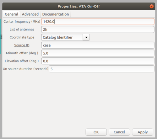
As was true for the simulated observation, if you'd like to use the On-Off block instead of the Track Scan block, almost all of the instructions for the Track Scan observation are equally applicable. Set up the flowgraph like this:
For the On-Off block, in addition to setting the center frequency, antennas list, and source location as you did before, for the On-Off block you will also need to indicate your on-source duration and the amount of offsets which you wish for the antenna to slew away from the source for the off-source part of the observation. Add an IF Switch block with the proper antennas selected as before.
When you play this flowgraph, the antenna(s) will first slew onto your target source, and will track on that source for the given duration, then slew off-source by the offset amount you indicated in the block's properties. The antenna(s) will stay on the offset source until you stop the flowgraph.
Tutorial 3: Data Collection
As mentioned above, once you have pointed your antenna(s) at a target source you can run a flowgraph to record data. There are two ways to do this -- one is to record the complex voltages straight from the USRP source block, which produces very large files but saves the phase information from the data; and the other is to do some DSP to the signal before recording if you are not concerned about preserving the phase information of the signal and would prefer to have a smaller filesize. In the first section below we're going to go over the first method.
Saving Raw Voltage Data
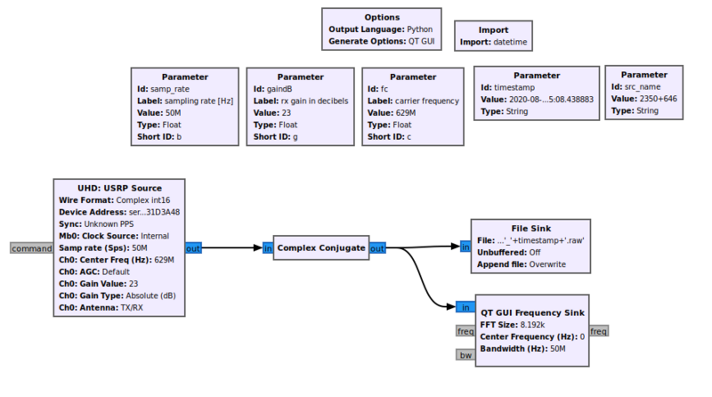
For this tutorial, please open the record_raw_data.grc example from the gr-ata examples folder in the GNU Radio companion. This example shows you how to record one polarization of data from a single antenna. The antenna you will be receiving data from will have been set by the antenna you selected in the IF Switch block when you ran the control flowgraph to point your antennas.
Before running the flowgraph, please make sure:
- You have set the right sampling rate in the samp_rate variable box. The USRPs can go up to 200 MS/s, or that number divided by any integer. The sample rate determines your bandwidth so be mindful of that (and also file size) when setting your sample rate.
- Make sure the center frequency in the fc variable box is set to 629 MHz; this ensures your USRP is recorded data centered on the LO frequency you indicated when you ran your flowgraph to initialize and point the antennas previously.
- Make sure src_name is set to the right identifier for your source. This doesn't affect your data, it just ensures you have a descriptive filename.
In the USRP source block, check that:
- The Device Address is set to "serial=31D3A48" to use the Ettus N321
- Mb0 Clock Source is set to internal
- Mb0 Subdev Spec is empty
- In RF Options, Antenna 0 is set to TX/RX
Note that the complex conjugate block in this flowgraph corrects for the fact that the raw voltages are flipped coming in to the system.
Now you can run the flowgraph! Note that if you start seeing OO's appear in the output you should stop recording and try reducing the sampling rate because in that case it is likely that you are saving data more quickly than the system can handle it.
If you are recording data successfully and not seeing OO's, just record for as long as you like and then click the Stop sign when you are finished.
It should not be too difficult to extend this example flowgraph to accept input from multiple channels and / or multiple USRPs.
Saving spectrum data
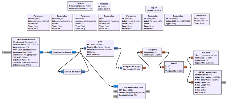
For this tutorial, please open the record_psd_data.grc flowgraph from the examples folder in GNU Radio companion. Setup for this type of data recording is, in many ways, similar to the initialization for recording raw data but there are a few additions.
As for the raw recording, make sure that in the USRP source block:
- The Device Address is set to "serial=31D3A48" to use the Ettus N321
- Mb0 Clock Source is set to internal
- Mb0 Subdev Spec is empty
- In RF Options, Antenna 0 is set to TX/RX
And also check that:
- You have set the right sampling rate in the samp_rate variable box. The USRPs can go up to 200 MS/s, or that number divided by any integer. The sample rate determines your bandwidth so be mindful of that (and also file size) when setting your sample rate.
- Make sure the center frequency in the fc variable box is set to 629 MHz; this ensures your USRP is recorded data centered on the LO frequency you indicated when you ran your flowgraph to initialize and point the antennas previously.
- Make sure src_name is set to the right identifier for your source. This doesn't affect your data, it just ensures you have a descriptive filename.
- Set the decimation variable to the number of vectors you want to integrate over. Higher decimation = better signal to noise and smaller filesize, but also lower time resolution in your resulting data.
- Set the fftsize variable to the number of points you want your FFT to be -- note it should be a power of 2. Note that the larger the fftsize, the better the spectral resolution but the lower the time resolution.
Once you are certain everything is set up properly, go ahead and run the flowgraph, and remember to turn it off when you are finished or you will accrue lots of data.
Tutorial 4: Playing back recorded data
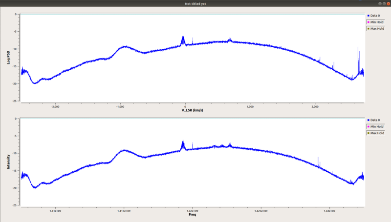
Since I've posted tutorials on how to record both raw and spectrum data, I'd like to now cover how to play back the data you've recorded and do some analysis on it. This tutorial will be split into two sections like Tutorial 3 as you will need to plot raw and spectrum data differently. Below is a sample plot showing an example of what the resulting plots from both methods will look like:
Note that the provided flowgraphs not only plot the results against frequency, but they also have the capability to plot the results converted to a velocity with respect to local standard of rest (V_LSR) if you have a need for it.
Plotting a spectrum from a raw data file
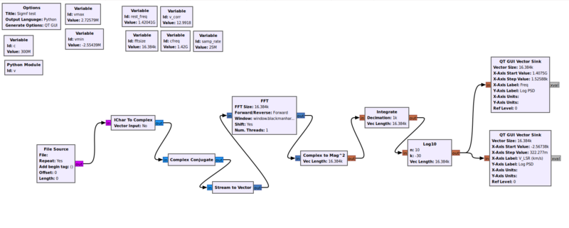
To plot a spectrum from a raw data file, you will need to do a bit of extra processing to get the raw data from voltage to power spectrum form; these processing steps are done by the blocks between the file source block and the vector sink block as shown below; this flowgraph can be found in examples under the name plot_from_raw.grc.
Of course the first step is to make sure you've selected the proper data file in the file sink block.
To process the data to your liking, make sure you have:
- Set the fftsize variable to the number of points you want your FFT to be -- note it should be a power of 2. Note that the larger the fftsize, the better the spectral resolution but the lower the time resolution.
- Set the decimation variable to the number of vectors you want to integrate over. Higher decimation = better signal to noise and smaller filesize, but also lower time resolution in your resulting data.
For the spectrum plot, it is important to make sure that you have:
- Set the cfreq equal to the value that your LO was set to during your observation (1420 MHz in this case).
- Set the samp_rate equal to the value of the sample rate used during recording
If you don't want to plot VLSR, just disable or delete that block. If you do, however, you must make sure to:
- Set the rest_freq to the rest frequency of the spectral line you want to observe.
- Open the variable v_corr, and in the function call (ie v.vlsr_correction('2010-03-26T15:16:33', 2.451075, 61.873500)) make sure the first field is a timestamp of the beginning of the observation in the same format as shown here (the filenames are automatically saved with the timestamp in their title); the second field is right ascension in hour angle and the third field is declination in decimal degrees.
At this point, if you have ensured everything is to your liking, you should be good to go to run the flowgraph and plot your data!
Plotting a spectrum from a pre-processed data file
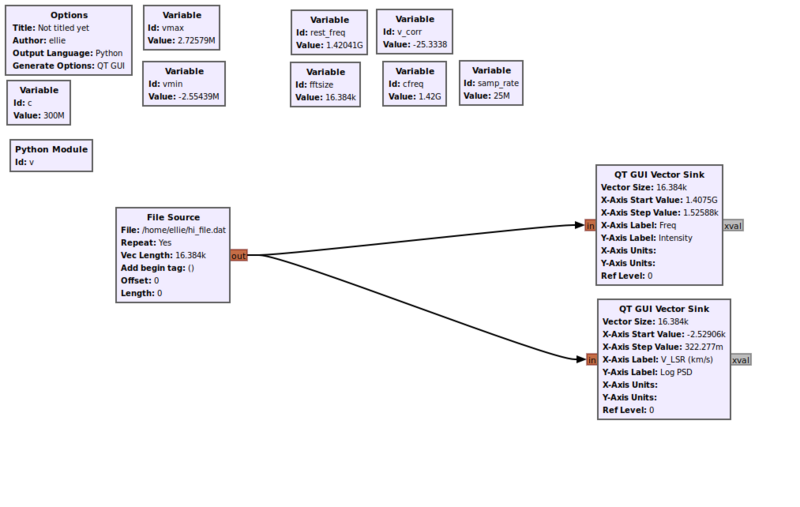
If you want to plot a spectrum from a data file which is already processed and saved in power spectrum format, the process is simpler. For this tutorial use the plot_from_psd.grc flowgraph found in examples.
Just make sure to:
- Enter the proper filepath in the File Sink block.
- Set the cfreq equal to the value that your LO was set to during your observation (1420 MHz in this case).
- Set the samp_rate equal to the value of the sample rate used during recording divided by two (since the samples are real, not complex).
Again, if you don't want to plot VLSR, just disable or delete that block. If you do, however, you must make sure to:
- Set the rest_freq to the rest frequency of the spectral line you want to observe.
- Open the variable v_corr, and in the function call (ie v.vlsr_correction('2010-03-26T15:16:33', 2.451075, 61.873500)) make sure the first field is a timestamp of the beginning of the observation in the same format as shown here (the filenames are automatically saved with the timestamp in their title); the second field is right ascension in hour angle and the third field is declination in decimal degrees.
Press play and you should be good to go!

