Creating Your First Block
This tutorial will guide you through creating your first block with the Embedded Python Block. The previous tutorial is here: Streams and Vectors
The example block we are creating will either add or multiply the two inputs based on a block parameter.
Opening Code Editor
The Embedded Python Block is a tool to quickly prototype a block within a flowgraph. Search for the Python Block and add it to the workspace:
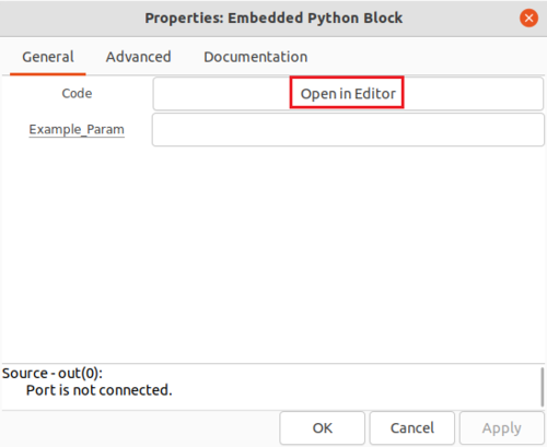
Double-click the box to edit the properties. The Embedded Python Block has two properties,
- Code, a click-box which contains a link to the Python code for the block and
- Example_Param, an input parameter to the block.
Click on Open in Editor to edit the Python code:
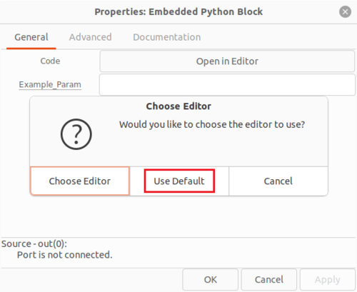
You will be prompted with another choice for which editor to use to write the Python code. Click Use Default:
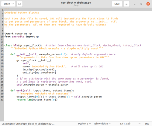
An editor window will then display the Python code for the Embedded Python Block:
Components of a Python Block
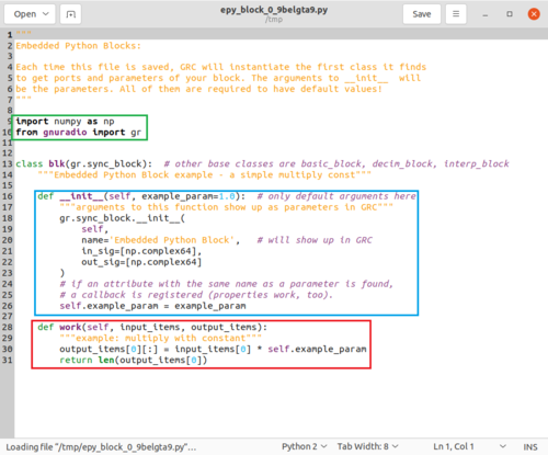
There are three important sections in the Python block code:
- import statements in green
- __init__ function in orange
- work function in red
The import statement includes the NumPy and GNU Radio libraries.
The __init__ statement:
- Accepts the example_param parameter with a default argument of 1.0
- Declares the block to have a np.complex64 input and output, which is the GNU Radio Complex Float 32 data type
- Stores the self.example_param variable from the input parameter
The work function:
- Has the input input_items and output output_items parameters
- Applies a mathematical operation to input_items and stores the result in output_items
- Returns the number of samples produced
Changing Parameter Name
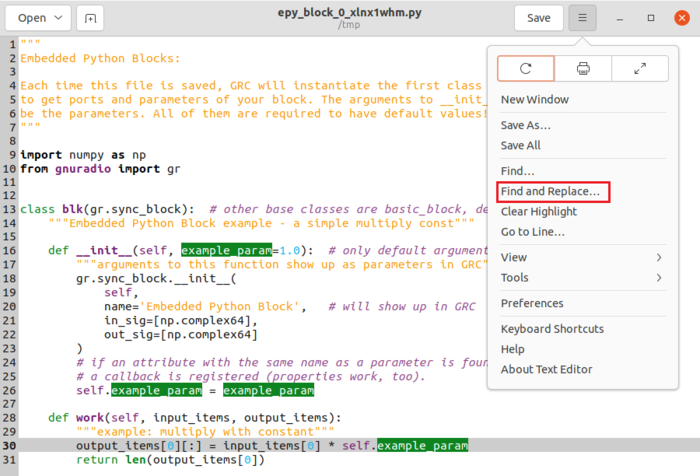
The first step will be to rename example_param to additionFlag to be more descriptive. From the editor menu select Find and Replace:
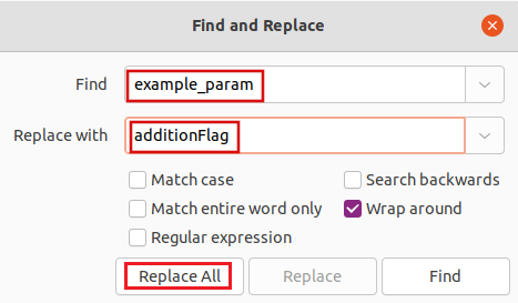
Enter example_param under Find, and additionFlag under Replace with, and then click Replace All:
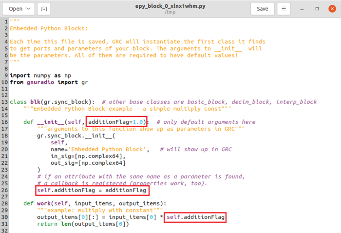
The parameter will be changed and the Python code will then look like this:
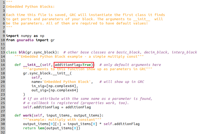
Now change the default value to be True:
Save the file:
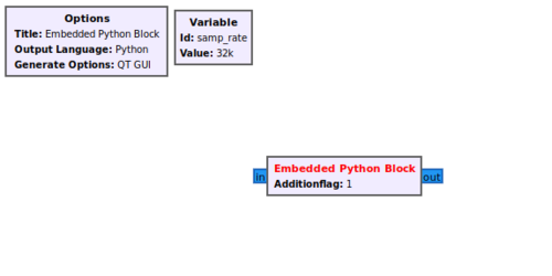
Return back to the GRC window and it will show that the block now displays the Additionflag parameter instead of example_param:
Editing Block Inputs
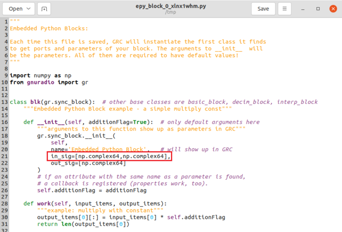
The default block has a single input and a single output, however we need two inputs for the block. To add an input, add a second np.complex64 to the in_sig list:
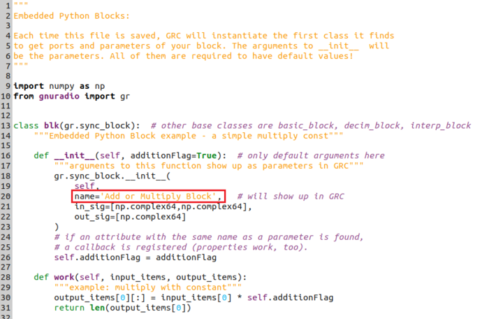
Now change the block name to Add or Multiply Block:
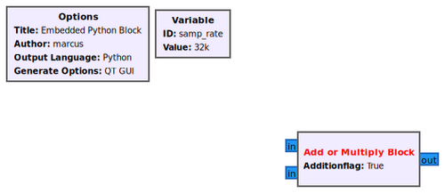
Save the file. GRC will now display the block with a second input and the block name will be updated:
Editing Work Function
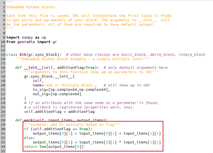
Now that the variable name has been changed the work function needs to be re-written to provide the desired functionality.
The pseudo code for the Python block is:
if (additionFlag is True)
    then add the two inputs
else
    then multiply the two inputs
Modify the work function so it has the following code:
Remember to indent with multiples of 4 spaces (4, 8, 12, etc.) when starting new lines in Python!
Save the the code.
Connecting the Flowgraph
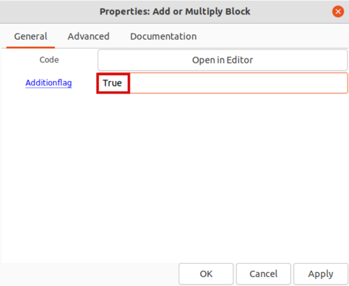
Return to GRC. Double-click the Add or Multiply Block. Enter True for the Additionflag property:
Click OK to save.
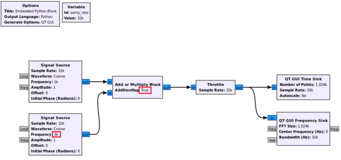
Drag and drop two Signal Source blocks, a Throttle block, a QT GUI Time Sink and a QT GUI Frequency Sink block into the GRC workspace and connect them according to the following flowgraph. Set the frequency of the second Signal Source to 3000:
Running the Flowgraph
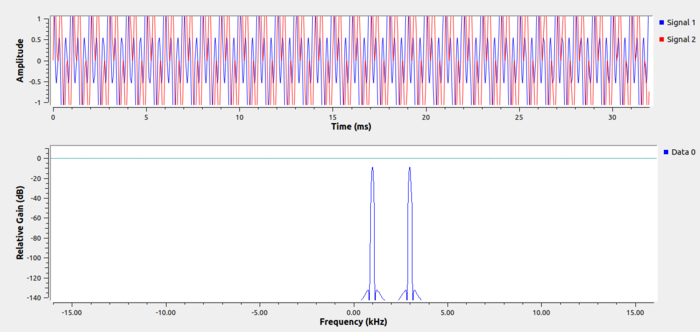
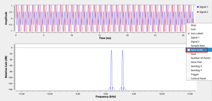
Selecting True in the Add or Multiply Block will perform the addition of the two Signal Sources. Running the flowgraph gives the following two plots:
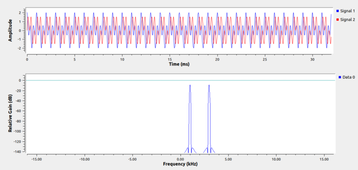
The plots show the summation of the two sinusoids, one at a frequency of 1,000 and another at 3,000. The y-axis in the QT GUI Time Sink plot is partially cutting of the amplitude of the sinusoids. Click the mouse-wheel button to bring up the display menu and select Auto Scale:
The full amplitude of the two sinusoids can then be seen:
Enter False for the Amplitudeflag property:
Click OK to save.
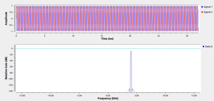
By definition, the multiplication of two complex sinusoids produces a sinusoid at the summation of the two frequencies. Therefore, the multiplication of the Signal Source of frequency 1,000 and frequency 3,000 will be a complex sinusoid of frequency 4,000. This complex sinusoid is seen when running the flowgraph:

