TutorialsSimulations
Simulations with GNU Radio
GNU Radio is not primarily intended for simulations, but often these are an important step in the development of signal processing code. Using GNU Radio can even be advantageous at times, since the simulation code and the code to actually transmit over the air is always the same.
When not to use GNU Radio as a simulation tool
There never is a reason that completely rules out GNU Radio as a simulation tool. However, there are situations when other tools might be suited better for the task, in particular when development time is an issue. If you're not planning to ever take your code live on the air, and just need simulations results e.g. to create graphs for a research paper, other tools might be more suitable.
Using the GNU Radio Companion
The GNU Radio Companion (GRC) is always a good choice to create flow graphs, provided that all the blocks you need are available in GRC (if you've written these blocks yourself, you might need to create GRC bindings by writing the *.xml files).
First, launch GRC by typing gnuradio-companion on a terminal or command line. This will launch the GRC graphical environment.
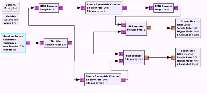
Here's an example of how GRC can be used to create a simulation environment. The following flow graph is available as part of the Channel Coding toolbox and was used to demonstrate the capabilities of the included Reed-Muller-Golay code. The original CGRAN server is offline, the code from the channel coding toolbox has been uploaded to github.com/ckuethe/gr-chancoding and is unlikely to work without some work to use newer GNU Radio APIs.
A very important thing to observe is the use of the throttle block (the first block after the random source). This block only allows a certain amount of bits to pass the block (this is not an exact rate, but the average rate of bits leaving this block will be the given sampling rate). If you omit the throttle block, you risk your CPU running the flow graph at full speed and eating up all of your computers processing power.
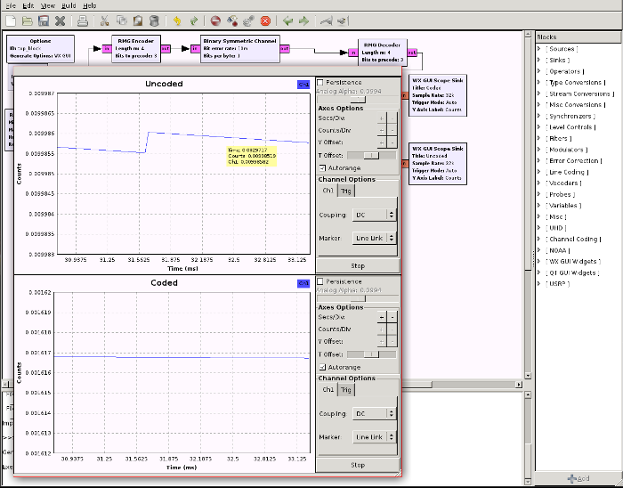
This flow graph uses graphical sinks to display the BER result in real time. As you can see, the BER is significantly lower for the coded path, which is exactly what you would expect.
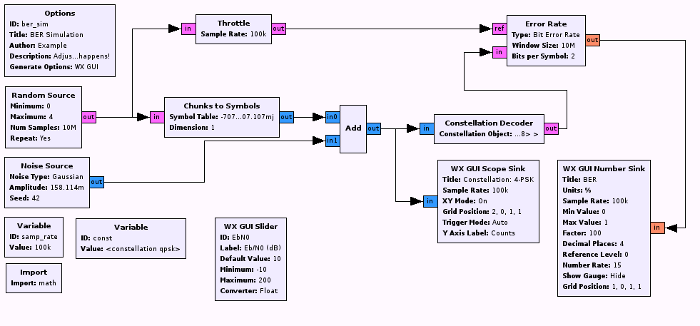
Another example is this BER simulator:
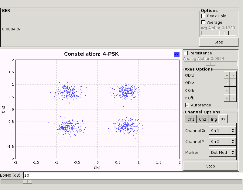
Again, it uses a throttle block to limit CPU usage. This flow graph adds AWGN to a complex constellation diagram; you can see how moving the Eb/N0 slider will increase or decrease the bit error rate.
Using vector sinks and sources
If you're running a typical simulation which repeats the exact same experiment many times, thereby slightly changing some parameter (e.g. SNR), this might be one of the rare cases when using Vector Sources and Sinks might be sensible (the other case being unit tests, which are essentially very similar).
In the above example, this is what you could do:
- Replace the random source with a vector source
- Replace the scope sinks with vector sinks
- Write a loop which restarts the flow graph for several different values of BER on the BSC
- For every loop iteration, put in a large number of bits in the vector source, run the flow graph and calculate the average of the elements in the vector sink. This would be your average BER at the receiver for a given BER on the channel.
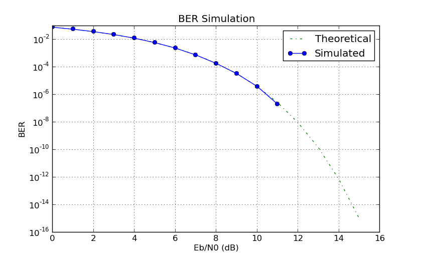
One example of this is source:gr-digital/examples/berawgn.py, which creates the following result:
Note that the flow graph used does not have a throttle block, but limits the CPU cycles with a head block. Such a block terminates execution after a certain number of items has passed, the flow graph thus does not run indefinitely.
