Sample Rate Tutorial: Difference between revisions
m (remove draft notation) |
|||
| (12 intermediate revisions by 3 users not shown) | |||
| Line 1: | Line 1: | ||
<!-- Sample_Rate_Tutorial.mediawiki --> | |||
== Demonstrate the effects of Sample Rate with GRC == | |||
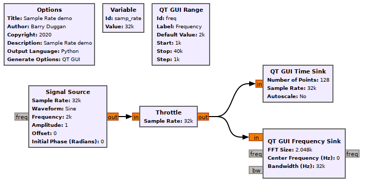
The following flowgraph will be used to demonstrate the effects of sample rate on signal processing. In this discussion, the [https://en.wikipedia.org/wiki/Nyquist%E2%80%93Shannon_sampling_theorem Nyquist-Shannon sampling theorem] establishes a minimum sampling rate of twice the signal frequency. Shannon's version of the theorem states: | |||
<blockquote> | |||
If a function <math>x(t)</math> contains no frequencies higher than <math>B</math> hertz, it is completely determined by giving its ordinates at a series of points spaced <math>1/(2B)</math> seconds apart. | |||
</blockquote> | |||
Note: the Sample Rate is set to 32 kHz. | |||
[[File:Samp_rate_demo_fg.png|900px]] | |||
=== Frequency: 2000 === | |||
With the frequency set at 2000, the time trace shows the expected sine wave, and the frequency plot shows a single signal at 2.0 kHz. | |||
[[File:Samp_rate_demo_out1.png|600px]] | |||
=== Frequency: 15000 === | |||
Setting the frequency to 15000, the frequency plot shows a single signal at 15.0 kHz, but the time trace shows significant degradation of the waveform. | |||
[[File:Samp_rate_demo_out2.png|600px]] | |||
=== Frequency: 18000 === | |||
Setting the frequency to 18000, the time trace not only shows significant degradation of the waveform, but the frequency plot shows a single signal at 14.0 kHz! This is called ''aliasing'', which is an artifact of insufficient sampling rate. | |||
[[File:Samp_rate_demo_out3.png|600px]] | |||
== Source hardware example == | |||
There are several factors which determine the rate at which data flows from one block to the next. However, many beginners assume that if, for example, a waveform source is set to a certain frequency, and a sample rate is set, then that output signal will be at that rate. But, as opposed to a hardware circuit, the signal is just data in a buffer. The following sections will illustrate this. | There are several factors which determine the rate at which data flows from one block to the next. However, many beginners assume that if, for example, a waveform source is set to a certain frequency, and a sample rate is set, then that output signal will be at that rate. But, as opposed to a hardware circuit, the signal is just data in a buffer. The following sections will illustrate this. | ||
This discussion is based on the flowgraph of a RadioTeleTYpe (RTTY) receiver. It can be found at [https://raw.githubusercontent.com/duggabe/gr-RTTY-basics/master/RTTY_rcv/RTTY_receive.grc] | |||
[[File:RTTY_rcv.png|960px]] | |||
Frequency shift keying (FSK) tones are input to the microphone jack of the computer which has a sample rate of 48 kHz. That data is fed to a Frequency Xlating FIR Filter which shifts the tones above and below the center frequency. It also decimates (divides) the sample rate by 50, producing an output sample rate of 960. | |||
The Quadrature Demod produces a signal which is positive or negative depending on whether the tone is above or below the center frequency. The gain is calculated by <code>samp_rate/(2*math.pi*fsk_deviation*decim)</code> which gives 0.898757 | |||
The | The RTTY symbol time is, by definition, exactly 22 ms. yielding the familiar 45 baud (1/0.022 rounded). To get an integer number of samples per symbol, a sample rate of 500 was chosen, producing 11 samples per symbol time. | ||
The Rational Resampler interpolates (multiplies) the sample rate by 500 and decimates it by 960 to produce an output sample rate of 500 | The output of the Quadrature Demod block has a sample rate of 960; the desired sample rate is 500. The Rational Resampler interpolates (multiplies) the sample rate by 500 and decimates (divides) it by 960 to produce an output sample rate of 500. | ||
The 'Terminal Display Sink' is an Embedded Python Block which reads the input stream of 1's and 0's, synchronizes on the start bit | The 'Terminal Display Sink' is an Embedded Python Block which reads the input stream of 1's and 0's, synchronizes on the start bit, creates a Baudot character from the five data bits, converts Baudot to UTF-8, and outputs the characters to a ZMQ PUSH Message Sink. | ||
== Sink hardware example == | == Sink hardware example == | ||
Whereas the example above is fairly straight forward, timing controlled by a hardware sink must be analyzed by starting at the output and working backwards through the flowgraph | Whereas the example above is fairly straight forward, timing controlled by a hardware sink must be analyzed by starting at the output and working backwards through the flowgraph! | ||
The following discussion is based on this flowgraph: | The following discussion is based on this flowgraph of a Morse Code generator: | ||
[[File:MorseGen_fg.png| | [[File:MorseGen_fg.png|900px]] | ||
For this example, the output Audio Sink has a sample rate of | For this example, the output Audio Sink has a sample rate of 48 kHz. This is fed by a Rational Resampler which interpolates (multiplies) the sample rate by 4, so the input sample rate must be 12000 (12 kHz). | ||
The Multiply, IIR Filter, and Uchar to Float blocks do not change the sample rate. | The Multiply, IIR Filter, and Uchar to Float blocks do not change the sample rate. | ||
The Repeat block takes each data item of input and repeats it 1200 times. This | The Repeat block takes each data item of input and repeats it 1200 times. (This is a form of interpolation.) This forces an input sample rate of 10, which is the desired baud rate. To provide for various code speeds, Variable blocks define the following: | ||
The <code>speed</code> variable in words per minute can be set by the user to any of the following: 2, 3, 4, 6, 8, 12, 16, or 24 (all are factors of 48). | The <code>speed</code> variable in words per minute can be set by the user to any of the following: 2, 3, 4, 6, 8, 12, 16, or 24 (all are factors of 48). | ||
| Line 37: | Line 67: | ||
The <code>samp_rate</code> variable = baud * repeat | The <code>samp_rate</code> variable = baud * repeat | ||
The 'Morse code vector source' is an Embedded Python Block which gets characters from the 'QT GUI Message Edit Box' and converts them into vectors, where each 1 is a dot bit time and each 0 is a space of one bit time. The complete description of Morse Code is | The 'Morse code vector source' is an Embedded Python Block which gets characters from the 'QT GUI Message Edit Box' and converts them into vectors, where each 1 is a dot bit time and each 0 is a space of one bit time. The complete description of Morse Code is given [https://en.wikipedia.org/wiki/Morse_code here]. The Morse Code generator project, including the flowgraph and Python code, can be found in [https://github.com/duggabe/gr-morse-code-gen gr-morse-code-gen]. | ||
== When there is no hardware block == | == When there is no hardware block == | ||
Some flowgraphs, such as for testing or simulation, do not involve any hardware devices to set a sample rate. In those cases a Throttle block can be used instead. | Some flowgraphs, such as for testing or simulation, do not involve any hardware devices to set a sample rate. In those cases a [[Throttle]] block can be used instead. | ||
'''[[Throttle]] is not adequate when the sampling rate is already defined by a sampling hardware device, like a sound card or an SDR frontend (USRP etc.)!''' | |||
[[Throttle]] simply slows down the ''processing'' of samples, and does nothing to the samples themselves. Since GNU Radio blocks can only process signal as long as there is some input in their input buffer(s) and as long as there is some space for the output in their output buffer(s), Throttle can effectively limit the throughput of a flow graph by limiting how many samples it copies from its own in- to its output, or by only consuming samples at a limited rate. | |||
This is very useful in situations where you want to look at a synthetic signal in a visualization: | |||
[[File:demonstrate_throttle.png]] | |||
This is an example from the [[Throttle]] block documentation. In the upper component, the rate at which the [[Signal Source]] can produce is limited by Throttle consuming them at the specified average rate. In the lower component, the other [[Signal Source]] is not limited by anything but how fast your CPU can produce data and shuffle it into the [[QT GUI Time Sink]] – leading to both a fully occupied CPU core just generating the signal, and a practically useless visualization in the "Unthrottled" Qt GUI Time Sink. | |||
Latest revision as of 15:12, 4 April 2024
Demonstrate the effects of Sample Rate with GRC
The following flowgraph will be used to demonstrate the effects of sample rate on signal processing. In this discussion, the Nyquist-Shannon sampling theorem establishes a minimum sampling rate of twice the signal frequency. Shannon's version of the theorem states:
If a function contains no frequencies higher than hertz, it is completely determined by giving its ordinates at a series of points spaced seconds apart.
Note: the Sample Rate is set to 32 kHz.
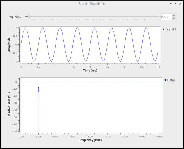
Frequency: 2000
With the frequency set at 2000, the time trace shows the expected sine wave, and the frequency plot shows a single signal at 2.0 kHz.
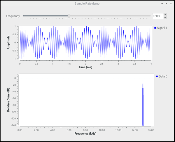
Frequency: 15000
Setting the frequency to 15000, the frequency plot shows a single signal at 15.0 kHz, but the time trace shows significant degradation of the waveform.
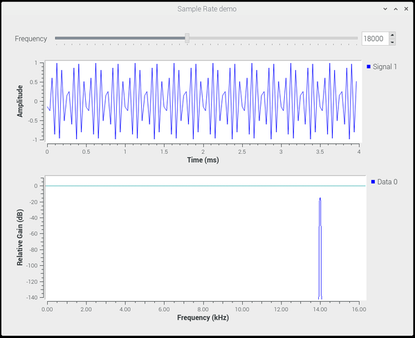
Frequency: 18000
Setting the frequency to 18000, the time trace not only shows significant degradation of the waveform, but the frequency plot shows a single signal at 14.0 kHz! This is called aliasing, which is an artifact of insufficient sampling rate.
Source hardware example
There are several factors which determine the rate at which data flows from one block to the next. However, many beginners assume that if, for example, a waveform source is set to a certain frequency, and a sample rate is set, then that output signal will be at that rate. But, as opposed to a hardware circuit, the signal is just data in a buffer. The following sections will illustrate this.
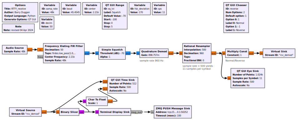
This discussion is based on the flowgraph of a RadioTeleTYpe (RTTY) receiver. It can be found at [1]
Frequency shift keying (FSK) tones are input to the microphone jack of the computer which has a sample rate of 48 kHz. That data is fed to a Frequency Xlating FIR Filter which shifts the tones above and below the center frequency. It also decimates (divides) the sample rate by 50, producing an output sample rate of 960.
The Quadrature Demod produces a signal which is positive or negative depending on whether the tone is above or below the center frequency. The gain is calculated by samp_rate/(2*math.pi*fsk_deviation*decim) which gives 0.898757
The RTTY symbol time is, by definition, exactly 22 ms. yielding the familiar 45 baud (1/0.022 rounded). To get an integer number of samples per symbol, a sample rate of 500 was chosen, producing 11 samples per symbol time.
The output of the Quadrature Demod block has a sample rate of 960; the desired sample rate is 500. The Rational Resampler interpolates (multiplies) the sample rate by 500 and decimates (divides) it by 960 to produce an output sample rate of 500.
The 'Terminal Display Sink' is an Embedded Python Block which reads the input stream of 1's and 0's, synchronizes on the start bit, creates a Baudot character from the five data bits, converts Baudot to UTF-8, and outputs the characters to a ZMQ PUSH Message Sink.
Sink hardware example
Whereas the example above is fairly straight forward, timing controlled by a hardware sink must be analyzed by starting at the output and working backwards through the flowgraph!
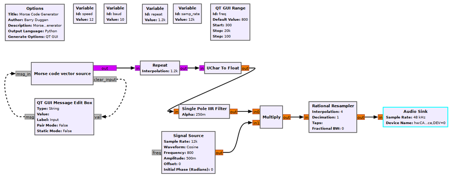
The following discussion is based on this flowgraph of a Morse Code generator:
For this example, the output Audio Sink has a sample rate of 48 kHz. This is fed by a Rational Resampler which interpolates (multiplies) the sample rate by 4, so the input sample rate must be 12000 (12 kHz).
The Multiply, IIR Filter, and Uchar to Float blocks do not change the sample rate.
The Repeat block takes each data item of input and repeats it 1200 times. (This is a form of interpolation.) This forces an input sample rate of 10, which is the desired baud rate. To provide for various code speeds, Variable blocks define the following:
The speed variable in words per minute can be set by the user to any of the following: 2, 3, 4, 6, 8, 12, 16, or 24 (all are factors of 48).
The baud variable = speed / 1.2
The repeat variable is fixed at 1200.
The samp_rate variable = baud * repeat
The 'Morse code vector source' is an Embedded Python Block which gets characters from the 'QT GUI Message Edit Box' and converts them into vectors, where each 1 is a dot bit time and each 0 is a space of one bit time. The complete description of Morse Code is given here. The Morse Code generator project, including the flowgraph and Python code, can be found in gr-morse-code-gen.
When there is no hardware block
Some flowgraphs, such as for testing or simulation, do not involve any hardware devices to set a sample rate. In those cases a Throttle block can be used instead.
Throttle is not adequate when the sampling rate is already defined by a sampling hardware device, like a sound card or an SDR frontend (USRP etc.)!
Throttle simply slows down the processing of samples, and does nothing to the samples themselves. Since GNU Radio blocks can only process signal as long as there is some input in their input buffer(s) and as long as there is some space for the output in their output buffer(s), Throttle can effectively limit the throughput of a flow graph by limiting how many samples it copies from its own in- to its output, or by only consuming samples at a limited rate.
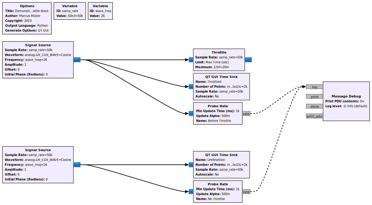
This is very useful in situations where you want to look at a synthetic signal in a visualization:
This is an example from the Throttle block documentation. In the upper component, the rate at which the Signal Source can produce is limited by Throttle consuming them at the specified average rate. In the lower component, the other Signal Source is not limited by anything but how fast your CPU can produce data and shuffle it into the QT GUI Time Sink – leading to both a fully occupied CPU core just generating the signal, and a practically useless visualization in the "Unthrottled" Qt GUI Time Sink.


