Sample Rate Tutorial

Adjusting the Sample Rate in GRC

We start with the flowgraph below:

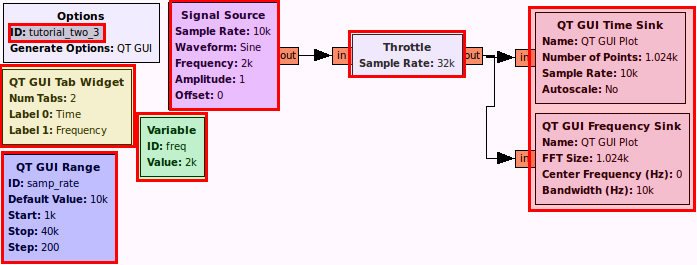
This flowgraph generates a sine wave and plots it in time and frequency. A slider allows us to dynamically adjust the sample rate while we hold the frequency of the sine wave constant.

The output looks like this:

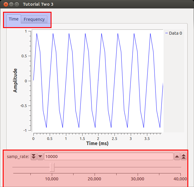
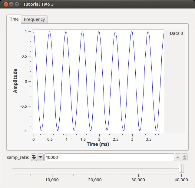
Our signal of the sine wave looks pretty bad with all those straight lines! What we can do is change the samp_rate variable without having to re-generate the flowgraph. Let's increase the samp_rate to the maximum by moving the slider fully to the right. Now we see the sine wave we would expect.

Testing the Nyquist Frequency

Now let's turn to the Frequency tab.

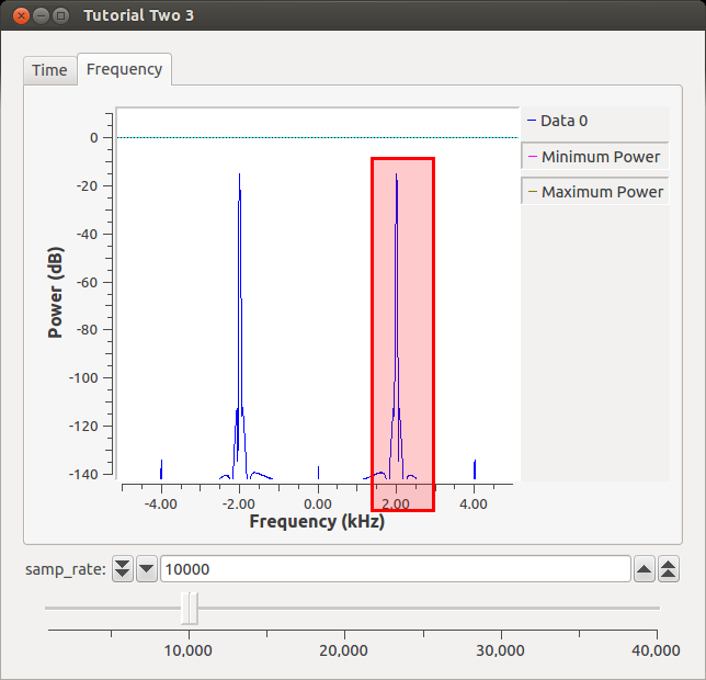
At a sampling rate of 10k, we are able to reproduce our original frequency (2 kHz). If we sample higher, we will still get a peak at 2 kHz. Nyquist tells us that once we sample at anything lower than 2*original_signal_freq, we will be unable to reproduce the signal. We read that in a textbook, though, so we are not convinced. Let's slide our samp_rate to 3.85 kHz. What happens to the Time waveform?

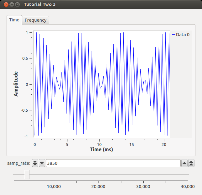
Well, it definitely doesn't look like a sine wave anymore, but our eyes can be deceived so let's turn to the FFT to get its frequency.

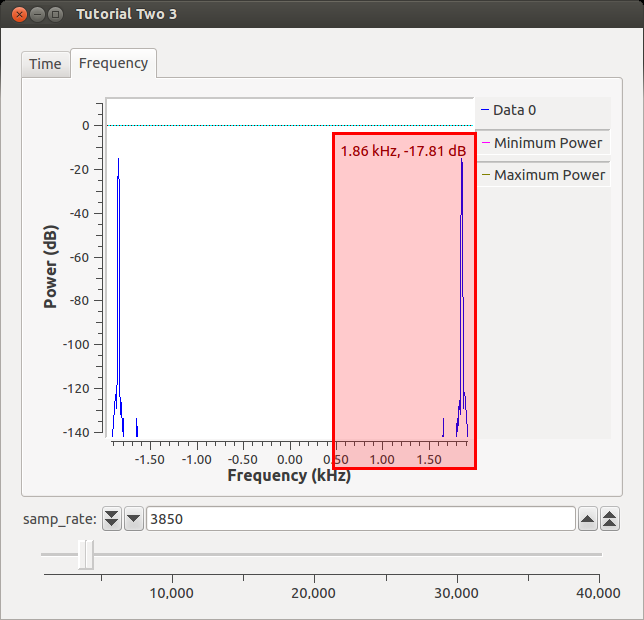
We see that the frequency is no longer at 2 kHz like it should be based on our input signal. Instead, since we are 0.15 kHz below the Nyquist rate, the signal has "folded-over" and is now 0.15 kHz below its actual frequency (my cursor was a little off :( ). This is simple sanity check that GNU Radio simulates DSP theory.

Source hardware example

There are several factors which determine the rate at which data flows from one block to the next. However, many beginners assume that if, for example, a waveform source is set to a certain frequency, and a sample rate is set, then that output signal will be at that rate. But, as opposed to a hardware circuit, the signal is just data in a buffer. The following sections will illustrate this.

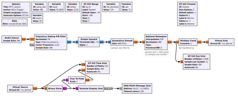
The following discussion is based on this flowgraph of a RadioTeleType (RTTY) receiver:

Frequency shift keying (FSK) tones are input to the microphone jack of the computer which has a sample rate of 48khz. That data is fed to a Frequency Xlating FIR Filter which shifts the tones above and below the center frequency. It also decimates (divides) the sample rate by 50, producing an output sample rate of 960.

The Quadrature Demod produces a signal which is positive or negative depending on whether the tone is above or below the center frequency.

The Rational Resampler interpolates (multiplies) the sample rate by 500 and decimates (divides) it by 960 to produce an output sample rate of 500. For the RTTY rate of 45.4545 baud (the exact definition is 1/0.022), this produces exactly 11 samples per bit time.

The 'Terminal Display Sink' is an Embedded Python Block which reads the input stream of 1's and 0's, synchronizes on the start bit, creates a Baudot character from the five data bits, converts Baudot to UTF-8, and displays the characters on the user terminal screen.

Sink hardware example

Whereas the example above is fairly straight forward, timing controlled by a hardware sink must be analyzed by starting at the output and working backwards through the flowgraph.

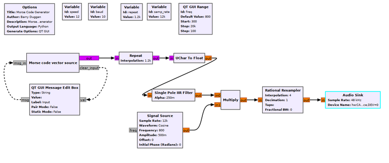
The following discussion is based on this flowgraph of a Morse Code generator:

For this example, the output Audio Sink has a sample rate of 48khz. This is fed by a Rational Resampler which interpolates (multiplies) the sample rate by 4, so the input sample rate must be 12000 (12khz).

The Multiply, IIR Filter, and Uchar to Float blocks do not change the sample rate.

The Repeat block takes each data item of input and repeats it 1200 times. (This is a form of interpolation.) This forces an input sample rate of 10, which is the desired baud rate. To provide for various code speeds, Variable blocks define the following:

The speed variable in words per minute can be set by the user to any of the following: 2, 3, 4, 6, 8, 12, 16, or 24 (all are factors of 48).

The baud variable = speed / 1.2

The repeat variable is fixed at 1200.

The samp_rate variable = baud * repeat

The 'Morse code vector source' is an Embedded Python Block which gets characters from the 'QT GUI Message Edit Box' and converts them into vectors, where each 1 is a dot bit time and each 0 is a space of one bit time. The complete description of Morse Code is given here.

When there is no hardware block

Some flowgraphs, such as for testing or simulation, do not involve any hardware devices to set a sample rate. In those cases a Throttle block can be used instead.

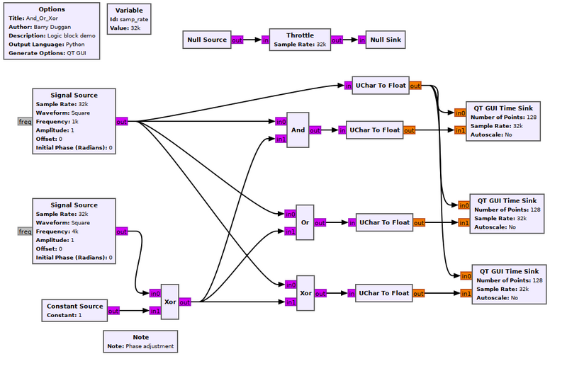
This flowgraph shows the usage of AND, OR, and XOR logic blocks. Since no hardware devices are involved, the Throttle block assures that the processor will not lock up trying to process the data at its maximum possible speed.

Note that the Throttle block doesn't even need to be in the 'main' data path to work.