User talk:Muaddib: Difference between revisions
No edit summary |
No edit summary |
||
| Line 40: | Line 40: | ||
For this Flowgraph, we will have an overall FFT size used to display our synthetic frequency spectrum. In this example it will be 8192 FFT bins. | For this Flowgraph, we will have an overall FFT size used to display our synthetic frequency spectrum. In this example it will be 8192 FFT bins. | ||
=Dumb Threshold= | ====Dumb Threshold==== | ||
For the 'dumb threshold', a vector where all values are adjustable will allow us to use a QT Range Widget to dynamically raise and lower the threshold. | For the 'dumb threshold', a vector where all values are adjustable will allow us to use a QT GUI Range Widget to dynamically raise and lower the threshold. | ||
This can be done by creating a QT Range Widget <code>thresh_adj</code> and entering <code>(thresh_adj,)*full_band_size</code> where <code>full_band_size</code> | This can be done by creating a QT GUI Range Widget <code>thresh_adj</code> and entering <code>(thresh_adj,)*full_band_size</code> where <code>full_band_size</code> | ||
has the value 8192, the overall FFT size for the flowgraph. | has the value 8192, the overall FFT size for the flowgraph. | ||
At runtime, the <code>thresh_adj</code> QT Range Widget will set all the indices of this vector to the same value which will display as a horizontal line spanning the entire | At runtime, the <code>thresh_adj</code> QT GUI Range Widget will set all the indices of this vector to the same value which will display as a horizontal line spanning the entire | ||
frequency window. When the variable is adjusted, the line moves up/down. | frequency window. When the variable is adjusted, the line moves up/down. | ||
=Frequency Boundary Box= | ====Frequency Boundary Box==== | ||
For the frequency boundary box, it gets a little more complicated. Consider a simple case of a vector with length 9, where the vector values are | For the frequency boundary box, it gets a little more complicated. Consider a simple case of a vector with length 9, where the vector values are | ||
<code>[-1000,-1000,-1000,-1000,+1000,-1000,-1000,-1000,-1000]</code> with indices <code>[0,1,2,3,4,5,6,7,8,9]</code>. | <code>[-1000,-1000,-1000,-1000,+1000,-1000,-1000,-1000,-1000]</code> with indices <code>[0,1,2,3,4,5,6,7,8,9]</code>. | ||
| Line 59: | Line 59: | ||
logic in with python expressions. | logic in with python expressions. | ||
For the Upper/Lower boundaries we will create vector sources where each vector will adjust it's left and right sides | For the Upper/Lower boundaries we will create vector sources where each vector will adjust it's left and right sides so that both of them combined will equal ''819'''1''''', adding the | ||
vertical line's index to the left and right sides will make the vector length add up to the FFT length '''8191+1=8192''' | vertical line's index to the left and right sides will make the total vector length add up to the FFT length '''8191+1=8192''' | ||
This section of the flowgraph is shown here: | |||
[[File:Two_vert_one_horiz_vectors.png]] | [[File:Two_vert_one_horiz_vectors.png]] | ||
| Line 78: | Line 78: | ||
<code>vec_height</code> is the extremely high value from our simple length 9 vector example (+1000) | <code>vec_height</code> is the extremely high value from our simple length 9 vector example (+1000) | ||
<code>low_line_adj</code> is a QT Range Widget that we use to adjust the position of the vertical line that indicates the lower frequency boundary of the frequency boundary box | <code>low_line_adj</code> is a QT GUI Range Widget that we use to adjust the position of the vertical line that indicates the lower frequency boundary of the frequency boundary box | ||
<code>up_line_adj</code> is a QT Range Widget that we use to adjust the position of the vertical line that indicates the upper frequency boundary of the frequency boundary box | <code>up_line_adj</code> is a QT GUI Range Widget that we use to adjust the position of the vertical line that indicates the upper frequency boundary of the frequency boundary box | ||
The upper and lower frequency boundary vectors will be constructed to expand or contract in length based on the desired position of their vertical boundary lines. | The upper and lower frequency boundary vectors will be constructed to expand or contract in length based on the desired position of their vertical boundary lines. | ||
| Line 87: | Line 87: | ||
The left half of the vector can be expressed as <code>(low_line_adj)*(below_zero,)</code>, which says that the number of bins to the left of the vertical line's position will be equal to the | The left half of the vector can be expressed as <code>(low_line_adj)*(below_zero,)</code>, which says that the number of bins to the left of the vertical line's position will be equal to the | ||
''position'' of the vertical line. So if the vertical line | ''position'' of the vertical line. So if the vertical line's position is index: 512, there will be 512 values to it's left (0-511) | ||
The right half of the vector can be expressed as <code>(fft_size-low_line_adj-1)*(below_zero,)</code>, which says the 'left side' of the vector will be equal to the number of bins | |||
between the vertical line's position index (512) and the rest of the total vector length 8192 (512-8192). We subtract 1 to account for the vertical line's position itself. | |||
When the vertical line position is adjusted with the QT GUI Range Widget, the left/right sides will adjust accordingly in real-time. The total will always be the overall FFT Length (8192). | |||
====Adding the synthetic signal to the Display==== | |||
Since the incoming signal is really the main event in spectrum monitoring, we should probably add that to the spectrum window. The 4th input (input 3) on the QT GUI Vector Sink is where we | |||
add our synthetic signal. In the section above, we showed how it can be constructed and summed together to create one stream of data, but now we need to also convert the time domain to a | |||
spectral representation. We do this by using the '''Low Power''' | |||
Revision as of 06:15, 22 August 2022
Application/Goals
Introduction
Sometimes a DSP application will call for signal detection of an intermittent signal (only present in the spectrum part of the time). A simplistic way to detect signal is by way of a frequency domain threshold, when an FFT bin exceeds that threshold the signal is 'detected'. Using a 'dumb' threshold would be a first obvious choice for triggering a detection event. The threshold level is the same across the entire spectral window and it is set to a value above the observed noisefloor, but below the minimum level of a particular signal we are trying to detect. With this simple approach (a straight line across the spectrum), a detection event is triggered anytime the threshold is exceeded. Ideally our threshold would only trigger on the specific signals we want to detect, those signals may be clustered together in frequency in a range or band contained within the spectral observation window. If we restrict the detection criteria to only a simple level threshold, some signals within our observation window may trigger a detection in error (since we only want to detect signals in a subband of our observation window) If we can restrict the threshold to not only power, but also frequency, we can still look at a large frequency range and see what else is present, but only trigger a detection if the threshold is crossed within the defined portion of spectrum.
Goals
Generate Synthetic RF Spectrum with Intermittent Carriers
- broadband noise
- narrowband signals with intermittent behavior
- a large wideband signal
Set Visual Boundary Lines around a segment of the Frequency Spectrum and a Threshold Level
- Visualize the Synthetic RF Spectrum in the Frequency Domain
- Create an adjustable threshold (horizontal line) that is displayed in the frequency window and also can be manually adjusted by the user.
- Add upper and lower frequency boundaries (vertical lines) which will restrict the threshold trigger to signals within the boundary box.
- use python conditional statements to trigger a file recording when the threshold is crossed (detection)
Generate 'Synthetic RF Spectrum'
In the following example we will: Generate a synthetic signal for testing. It is assumed that you are comfortable enough in GNURadio to understand what these blocks are doing.
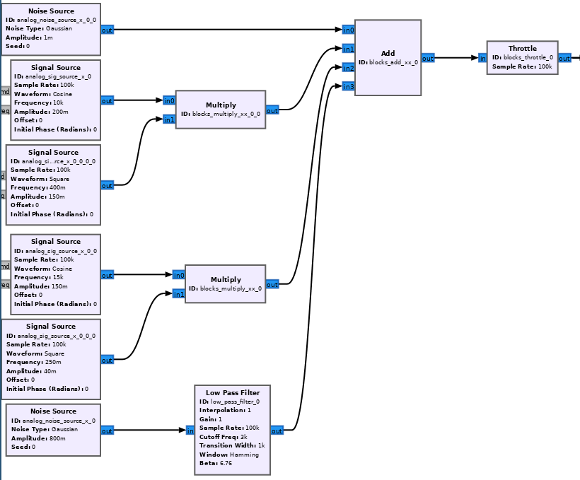
This portion of the flowgraph:
- generates gaussian noise for the overall noisefloor (simulating environmental broadband noise)
- Simulates a wideband carrier by lowpass filtering a noise source that is uncorrelated with the noise in the overall spectrum
- Creates two narrowband carriers which are each modulated by square waves of different frequencies to simulate intermittent transmissions
Create A Visual Utility to Set Detection Boundaries for Frequency and Level
This portion of the flowgraph is where we get creative with Vectors.
For this Flowgraph, we will have an overall FFT size used to display our synthetic frequency spectrum. In this example it will be 8192 FFT bins.
Dumb Threshold
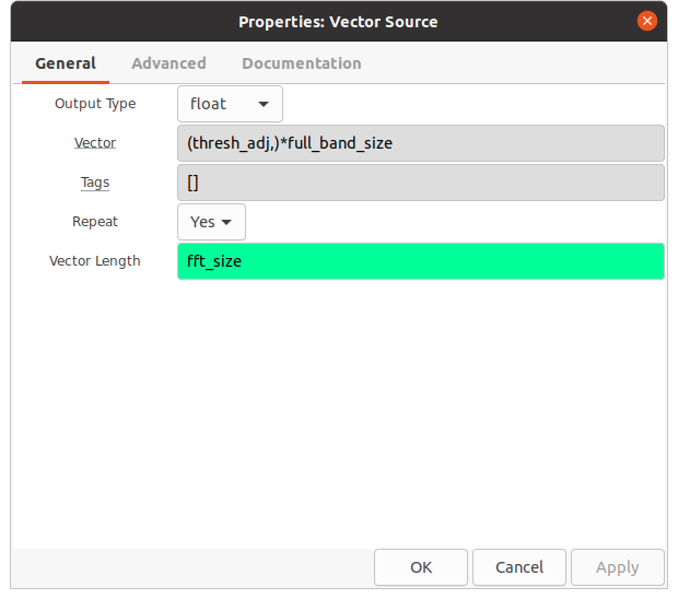
For the 'dumb threshold', a vector where all values are adjustable will allow us to use a QT GUI Range Widget to dynamically raise and lower the threshold.
This can be done by creating a QT GUI Range Widget thresh_adj and entering (thresh_adj,)*full_band_size where full_band_size
has the value 8192, the overall FFT size for the flowgraph.
At runtime, the thresh_adj QT GUI Range Widget will set all the indices of this vector to the same value which will display as a horizontal line spanning the entire
frequency window. When the variable is adjusted, the line moves up/down.
Frequency Boundary Box
For the frequency boundary box, it gets a little more complicated. Consider a simple case of a vector with length 9, where the vector values are
[-1000,-1000,-1000,-1000,+1000,-1000,-1000,-1000,-1000] with indices [0,1,2,3,4,5,6,7,8,9].
On a plot, we get a shape like this ____|____ where the flat parts across the bottom are 4 values of -1000 (index 0-3) on the left and 4 values of -1000 on the right (index 5-8) with one value in the middle (index 4) with value +1000. In GNURadio when we represent baseband samples as RF signals in the frequency domain (QT Frequency Sink) we limit the y-axis of the observation window to defaults of +10dB and -140dB, because we won't likely be able to receive signals greater than say +20 on a relative scale with common A/D's in SDR's. Therefore, if we insert a vector into a QT Vector GUI with values that exceed our viewing window, we will only see a vertical line in the window for the value of +1000. We can use that line as a boundary using some array logic in with python expressions.
For the Upper/Lower boundaries we will create vector sources where each vector will adjust it's left and right sides so that both of them combined will equal 8191, adding the vertical line's index to the left and right sides will make the total vector length add up to the FFT length 8191+1=8192
This section of the flowgraph is shown here:
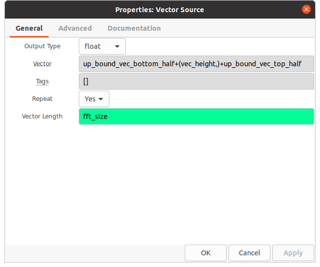
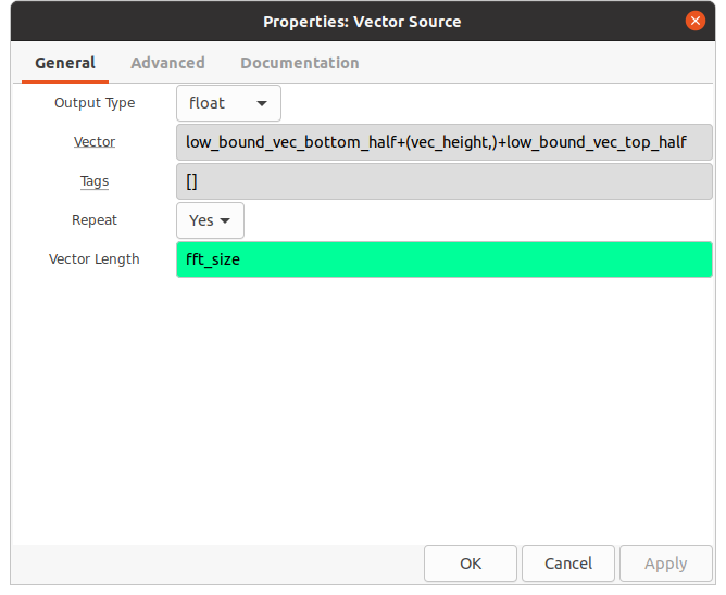
The parameters for the 3 Vector Source blocks are shown here:
fft_size = 8192
below_zero is the extremely low value from our simple length 9 vector example (-1000)
vec_height is the extremely high value from our simple length 9 vector example (+1000)
low_line_adj is a QT GUI Range Widget that we use to adjust the position of the vertical line that indicates the lower frequency boundary of the frequency boundary box
up_line_adj is a QT GUI Range Widget that we use to adjust the position of the vertical line that indicates the upper frequency boundary of the frequency boundary box
The upper and lower frequency boundary vectors will be constructed to expand or contract in length based on the desired position of their vertical boundary lines.
Both vertical boundary lines follow the same logic. In the case of the lower boundary line:
The left half of the vector can be expressed as (low_line_adj)*(below_zero,), which says that the number of bins to the left of the vertical line's position will be equal to the
position of the vertical line. So if the vertical line's position is index: 512, there will be 512 values to it's left (0-511)
The right half of the vector can be expressed as (fft_size-low_line_adj-1)*(below_zero,), which says the 'left side' of the vector will be equal to the number of bins
between the vertical line's position index (512) and the rest of the total vector length 8192 (512-8192). We subtract 1 to account for the vertical line's position itself.
When the vertical line position is adjusted with the QT GUI Range Widget, the left/right sides will adjust accordingly in real-time. The total will always be the overall FFT Length (8192).
Adding the synthetic signal to the Display
Since the incoming signal is really the main event in spectrum monitoring, we should probably add that to the spectrum window. The 4th input (input 3) on the QT GUI Vector Sink is where we add our synthetic signal. In the section above, we showed how it can be constructed and summed together to create one stream of data, but now we need to also convert the time domain to a spectral representation. We do this by using the Low Power


