Reading and Writing Binary Files: Difference between revisions
No edit summary |
(adding missing commas) |
||
| (9 intermediate revisions by the same user not shown) | |||
| Line 1: | Line 1: | ||
<div style="float:right"> | |||
{{Template:BeginnerTutorials}} | |||
</div> | |||
Binary files allow RF information to be recorded for offline usage. Before continuing it is useful to refer to the tutorial [[Signal Data Types]] which describes different data types in GNU Radio. | Binary files allow RF information to be recorded for offline usage. Before continuing it is useful to refer to the tutorial [[Signal Data Types]] which describes different data types in GNU Radio. | ||
The previous tutorial, [[Frequency_Shifting|Frequency Shifting]], describes how to change the frequency of a signal both mathematically and with DSP blocks. The next tutorial, [[RTL-SDR_FM_Receiver|RTL-SDR FM Receiver]], describes how to build a broadcast FM receiver using an RTL-SDR receiver. | |||
=Binary Data File Formats for DSP= | |||
==Data File Formats== | ==Data File Formats== | ||
| Line 5: | Line 13: | ||
Each binary file will have a specific data format, with the two most common being 32-bit floats and 16-bit integers. RF samples can be both positive and negative, and therefore all integers will be implied to be signed integers, for simplicity. The binary file will save all samples in the same format back to back. For example, a binary file of 16-bit integers will save sample 0 as 16 bits, then sample 1 as 16-bits, sample 2 as 16-bits, and so on. | Each binary file will have a specific data format, with the two most common being 32-bit floats and 16-bit integers. RF samples can be both positive and negative, and therefore all integers will be implied to be signed integers, for simplicity. The binary file will save all samples in the same format back to back. For example, a binary file of 16-bit integers will save sample 0 as 16 bits, then sample 1 as 16-bits, sample 2 as 16-bits, and so on. | ||
< | <pre> | ||
[ sample 0: 16 bit int ][ sample 1: 16 bit int ][ sample 2: 16 bit int ] ... | [ sample 0: 16 bit int ][ sample 1: 16 bit int ][ sample 2: 16 bit int ] ... | ||
</ | </pre> | ||
For example, a binary file of 32-bit floats will save sample 0 as 32 bits, then sample 1 as 32-bits, sample 2 as 32-bits, and so on. | For example, a binary file of 32-bit floats will save sample 0 as 32 bits, then sample 1 as 32-bits, sample 2 as 32-bits, and so on. | ||
< | <pre> | ||
[ sample 0: 32 bit float ][ sample 1: 32 bit float ][ sample 2: 32 bit float ] ... | [ sample 0: 32 bit float ][ sample 1: 32 bit float ][ sample 2: 32 bit float ] ... | ||
</ | </pre> | ||
==Real and Complex Formats== | ==Real and Complex Formats== | ||
| Line 19: | Line 27: | ||
RF samples can be either real or complex. When a real sample is saved to a binary file each sample is saved in order: sample 0, then sample 1, then sample 2, and so on. | RF samples can be either real or complex. When a real sample is saved to a binary file each sample is saved in order: sample 0, then sample 1, then sample 2, and so on. | ||
< | <pre> | ||
[ real sample 0 ][ real sample 1 ][ real sample 2 ] ... | [ real sample 0 ][ real sample 1 ][ real sample 2 ] ... | ||
</ | </pre> | ||
A complex sample, I + jQ, has both a real component (I) and imaginary component (Q). The I and Q components of each sample will be interleaved when saved to a binary file. I of sample 0, then Q of sample 0, then I of sample 1, then Q of sample 1, then I of sample 2, then Q of sample 2, and so on. | A complex sample, I + jQ, has both a real component (I) and imaginary component (Q). The I and Q components of each sample will be interleaved when saved to a binary file. I of sample 0, then Q of sample 0, then I of sample 1, then Q of sample 1, then I of sample 2, then Q of sample 2, and so on. | ||
< | <pre> | ||
[ I sample 0 ][ Q sample 0 ][ I sample 1 ][ Q sample 1 ][ I sample 2 ][ Q sample 2 ] ... | [ I sample 0 ][ Q sample 0 ][ I sample 1 ][ Q sample 1 ][ I sample 2 ][ Q sample 2 ] ... | ||
</ | </pre> | ||
==Saving Samples as Binary Files== | ==Saving Samples as Binary Files== | ||
| Line 39: | Line 47: | ||
Real samples stored as 16-bit integers: | Real samples stored as 16-bit integers: | ||
< | <pre> | ||
[ sample 0: 16 bit int ][ sample 1: 16 bit int ][ sample 2: 16 bit int ] ... | [ sample 0: 16 bit int ][ sample 1: 16 bit int ][ sample 2: 16 bit int ] ... | ||
</ | </pre> | ||
Real samples stored as 32-bit floats: | Real samples stored as 32-bit floats: | ||
< | <pre> | ||
[ sample 0: 32 bit float ][ sample 1: 32 bit float ][ sample 2: 32 bit float ] ... | [ sample 0: 32 bit float ][ sample 1: 32 bit float ][ sample 2: 32 bit float ] ... | ||
</ | </pre> | ||
Complex samples stored as interleaved 16-bit integers: | Complex samples stored as interleaved 16-bit integers: | ||
< | <pre> | ||
[ I sample 0: 16 bit int ][ Q sample 0: 16 bit int ][ I sample 1: 16 bit int ][ Q sample 1: 16 bit int ][ I sample 2: 16 bit int ][ Q sample 2: 16 bit int ] ... | [ I sample 0: 16 bit int ][ Q sample 0: 16 bit int ][ I sample 1: 16 bit int ][ Q sample 1: 16 bit int ][ I sample 2: 16 bit int ][ Q sample 2: 16 bit int ] ... | ||
</ | </pre> | ||
Complex samples stored as interleaved 32-bit floats: | Complex samples stored as interleaved 32-bit floats: | ||
< | <pre> | ||
[ I sample 0: 32 bit float ][ Q sample 0: 32 bit float ][ I sample 1: 32 bit float ][ Q sample 1: 32 bit float ][ I sample 2: 32 bit float ] [ Q sample 2: 32 bit float ] ... | [ I sample 0: 32 bit float ][ Q sample 0: 32 bit float ][ I sample 1: 32 bit float ][ Q sample 1: 32 bit float ][ I sample 2: 32 bit float ] [ Q sample 2: 32 bit float ] ... | ||
</ | </pre> | ||
==Endianness== | ==Endianness== | ||
| Line 67: | Line 75: | ||
For example, consider the hexadecimal value 0xABCD0123. A big endian system would store the value into memory by: | For example, consider the hexadecimal value 0xABCD0123. A big endian system would store the value into memory by: | ||
< | <pre> | ||
Data Value: [ 0xAB ] [ 0xCD] [ 0x01 ] [ 0x23 ] | Data Value: [ 0xAB ] [ 0xCD] [ 0x01 ] [ 0x23 ] | ||
Memory Address: [ 0x00 ] [ 0x01] [ 0x02 ] [ 0x03 ] | Memory Address: [ 0x00 ] [ 0x01] [ 0x02 ] [ 0x03 ] | ||
</ | </pre> | ||
A little endian system stores the bytes in the reversed order into memory: | A little endian system stores the bytes in the reversed order into memory: | ||
< | <pre> | ||
Data Value: [ 0x23 ] [ 0x01] [ 0xCD ] [ 0xAB ] [BR] | Data Value: [ 0x23 ] [ 0x01] [ 0xCD ] [ 0xAB ] [BR] | ||
Memory Address: [ 0x00 ] [ 0x01] [ 0x02 ] [ 0x03 ] | Memory Address: [ 0x00 ] [ 0x01] [ 0x02 ] [ 0x03 ] | ||
</ | </pre> | ||
Converting between endianness is sometimes referred to as a “byte swap” operation. The [[Endian_Swap|Endian Swap]] block performs this endian conversion. | Converting between endianness is sometimes referred to as a “byte swap” operation. The [[Endian_Swap|Endian Swap]] block performs this endian conversion. | ||
| Line 83: | Line 91: | ||
The '''File Sink''' block takes incoming samples and saves them to local storage. It is recommended to review the [[Signal Data Types]], [[Binary Files for DSP]] tutorials and the [[File_Sink|File Sink]] block page before continuing. | The '''File Sink''' block takes incoming samples and saves them to local storage. It is recommended to review the [[Signal Data Types]], [[Binary Files for DSP]] tutorials and the [[File_Sink|File Sink]] block page before continuing. | ||
=Writing Binary Files= | |||
==Block Options for Data Types== | ==Block Options for Data Types== | ||
| Line 318: | Line 328: | ||
[[File:Storing_binary_files_select_append.png]] | [[File:Storing_binary_files_select_append.png]] | ||
=Reading Binary Files= | |||
This tutorial describes how to read binary files using the '''File Source''' block along side how to diagnose potential errors. | |||
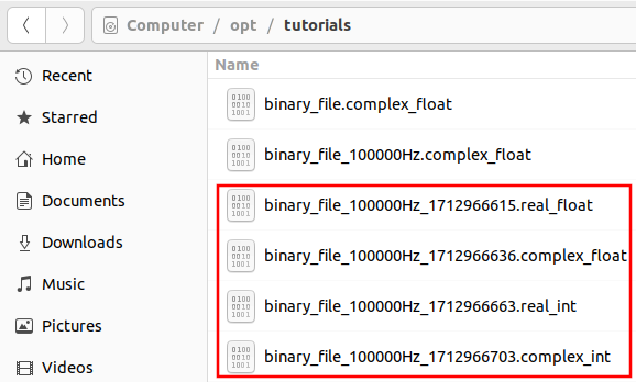
Please review the [[Writing_Binary_Files|Writing Binary Files]] tutorial before continuing. A series of binary files were created with different formats that will be needed for this tutorial: | |||
[[File:Reading_binary_files_all_formats.png]] | |||
==File Source Block== | |||
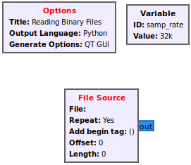
The '''File Source''' block reads from a binary file and then sends the samples to the output port. Drag the '''File Source''' block into a flowgraph. The block by default uses the complex data type (32-bit floats), represented by the '''<span style="color:blue">blue</span>''' output port: | |||
[[File:Reading_binary_files_add_file_sink_block.png]] | |||
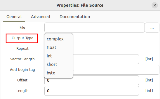
Double clicking the '''File Source''' block brings up the properties and the ability to select different data types. | |||
[[File:Reading_binary_files_file_source_data_types.png]] | |||
A binary file of real floating point data requires the float data type to be selected, which outputs real floating point samples, denoted by an '''<span style="color:orange">orange</span>''' output port. | |||
[[File:Reading_binary_files_file_sink_real_float.png]] | |||
A binary file of 16-bit signed integers requires the short data type to be selected, which outputs 16-bit integers of either real or interleaved I and Q samples (more on this later in the tutorial), denoted by a '''<span style="color:yellow">yellow</span>''' output port. | |||
[[File:Reading_binary_files_file_sink_real_short.png]] | |||
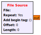
Also note that the '''File Source''' has the ''Repeat'' field enabled as ''Yes'', which will continually and repeatedly play back the same file. Once the last sample is received in the file it skips back to the first sample in the file and continues cycling through the file. | |||
[[File:Reading_binary_files_repeat_yes.png]] | |||
==Reading Complex Float== | |||
Add a '''File Source''' block, open the properties and begin by selecting the complex type. | |||
[[File:Reading_binary_files_add_complex_float_file_source.png]] | |||
Click the three dots to the right side of the File property to browse to a stored binary file. | |||
[[File:Reading_binary_files_open_file.png]] | |||
Select the file ending in ''.complex_float'': | |||
[[File:Reading_binary_files_select_complex_float.png]] | |||
The '''File Source''' block will now populate the filename: | |||
[[File:Reading_binary_files_complex_float_with_filename.png]] | |||
Notice that the filename is now filled in for the '''File Source''' however the ''samp_rate'' variable is incorrectly 32 kHz (32,000). The sampling rate from the filename is 100 kHz (100,000) therefore update the ''samp_rate'' variable: | |||
[[File:Reading_binary_files_update_samp_rate.png]] | |||
The change will be reflected in the flowgraph: | |||
[[File:Reading_binary_file_update_samp_rate_flowgraph.png]] | |||
Add in the '''QT GUI Time Sink''' and '''QT GUI Frequency Sink''' and connect them accordingly. Notice how both blocks use ''samp_rate'' variable automatically: | |||
[[File:Reading_binary_files_add_time_freq_sink.png]] | |||
Before running the flowgraph, recall that the [[Writing_Binary_Files|Writing Binary Files]] generated a 1 kHz complex sinusoid at a sampling rate of 100 kHz. When playing the file using the '''File Source''' the same waveform should be seen. | |||
[[File:Reading_binary_files_signal_source.png]] | |||
Now run the flowgraph. Notice that the time-domain plot has sinusoidal shapes on the I and Q channels, characteristic of a complex sinusoid. Also notice how the frequency plot displays a tone with a single peak, also characteristic of a complex sinusoid. Finally, notice how the peak of the frequency plot has a peak of approximately 1 kHz confirming that the binary file was read properly and the ''samp_rate'' variable was set properly. | |||
[[File:Reading_binary_files_time_freq_complex_float_display.png|750px]] | |||
==Reading Real Float== | |||
To read from a file storing real samples encoded as floating point numbers, open the '''File Source''' and change the ''Output Type'' to float: | |||
[[File:Reading_binary_files_select_real_float_type.png]] | |||
Click the three dots next to File and select the file ending in ''.real_float'': | |||
[[File:Reading_binary_files_select_real_float_file.png]] | |||
Open the '''QT GUI Time Sink''' properties and change the type to ''float'': | |||
[[File:Reading_binary_files_time_sink_real.png]] | |||
Open the '''QT GUI Freq Sink''' properties and change the type to ''float'': | |||
[[File:Reading_binary_files_freq_sink_real.png]] | |||
The flowgraph should now look like the following: | |||
[[File:Reading_binary_files_real_float_flowgraph.png]] | |||
Run the flowgraph. Notice that the time-domain plot displays a single sinusoid, characteristic of a real sinusoid waveform. Also notice that the frequency domain plot displays two peaks, characteristic of a real sinusoid. Finally, notice that the peak on the right hand side, the positive frequencies, is at approximately 1 kHz, confirming that the binary file was read properly and the ''samp_rate'' variable is set properly. | |||
[[File:Reading_binary_files_time_freq_real_float_display.png|750px]] | |||
==Reading Real Integers== | |||
Begin by adding a '''File Source''' block. Open the properties and navigate to the file ending in ''.real_int'': | |||
[[File:Reading_binary_files_select_real_int_file.png]] | |||
Change the ''Output Type'' property to be ''short''. '''Be sure not to select int''': | |||
[[File:Reading_binary_files_select_real_short_type.png]] | |||
Add in a Short to Float block and connect it accordingly: | |||
[[File:Reading_binary_files_real_int_flowgraph.png]] | |||
Notice that the scale factor here is set to 1. This will plot all of the values at full scale, which is from <math>-2^{15}</math> to <math>2^{15}-1</math>, or 32,768 to +32767. Running the flowgraph with a scaling value of 1 is valid, although some flowgraphs may use a scale factor in order to normalize the data to be within -1 to +1. Open the '''Short to Float''' properties and enter a scale factor of 2^15: | |||
[[File:Reading_binary_files_short_to_float_scale_factor.png]] | |||
The '''Short to Float''' block applies the inverse of the scale factor, meaning it will scale the output samples by <math>2^{-15}</math> or 1/32768. The flowgraph will now look like the following: | |||
[[File:Reading_binary_files_real_int_flowgraph_with_scale_factor.png]] | |||
Running the flowgraph displays the file after being read as real integers. The time domain plot displays a single sinusoid which is characteristic of a real sinusoid, and the frequency domain plot displays two tones which is also characteristic of a real sinusoid. Finally, the peak at the positive frequency tone is approximately 1 kHz which confirms that the file is being read correctly. | |||
[[File:Reading_binary_files_time_freq_real_int.png|750px]] | |||
==Reading Complex Integers== | |||
Begin by adding a '''File Source''' block. Open the properties and navigate to the file ending in ''.complex_int'': | |||
[[File:Reading_binary_files_select_complex_int.png]] | |||
Open the '''File Source''' properties and select the short data type. '''Do not select the int type''': | |||
[[File:Reading_binary_files_select_short_type.png]] | |||
Drag in a '''IShort to Complex''' block and connect it accordingly. Convert the '''QT GUI Time Sink''' and '''QT GUI Frequency Sink''' blocks into the ''complex'' data type. The flowgraph should look like the following. | |||
[[File:reading_binary_files_complex_int_flowgraph.png]] | |||
Note that the '''IShort to Complex''' block has a scale factor of 1, which would plot the data on a range of <math>-2^{15}</math> to <math>2^{15}-1</math>, or -32,768 to +32,767. Running the flowgraph in this state is valid. However, some flowgraphs require normalization such that all values are within -1 and +1. To do so, open the block’s properties and use a scale factor of <math>2^{15}</math>: | |||
[[File:Reading_binary_files_ishort_to_complex_scale_factor.png]] | |||
The '''IShort to Complex''' block will apply the inverse of the scale factor, <math>2^{-15}</math> or 1/32768, producing normalized samples from -1 to +1. | |||
[[File:Reading_binary_files_complex_int_flowgraph_scale_factor.png]] | |||
Run the flowgraph. The time domain plot displays two sinusoids, characteristic of a complex sinusoid. The frequency domain plot displays a single tone, also characteristic of a complex sinusoid. Finally, the tone is at approximate 1 kHz which confirms that the file is being read correctly. | |||
[[File:Reading_binary_files_time_freq_complex_int_display.png|750px]] | |||
==Continuous Playback from File== | |||
The '''File Source''' block comes with the option to repeat playback from file. When ''Yes'' is selected for repeat, the samples will be played back on loop until the flowgraph is stopped. | |||
[[File:Reading_binary_files_repeat_yes.png]] | |||
When ''No'' is selected for repeat, then all of the samples will be read from file and then the flowgraph will stop running once the last sample is read and then processed through the flowgraph. | |||
[[File:Reading_binary_files_repeat_no.png]] | |||
==Diagnosing Errors: Wrong Type and Format== | |||
In order to properly read a binary file both the type (real or complex) and format (integer or floating point) need to be known. If given a file and the type or format is unknown, it is best to check all possible combinations and to see which is the most reasonable. Endianness (described in the next section) is another potential problem when reading binary files. | |||
The following are examples of a file being read improperly. Warning: different recordings will present different type and format errors differently, '''the images presented here are not exhaustive''' and are only a couple of examples to help build intuition to diagnose these kinds of errors. | |||
The following image is an example of a real integer being read as real floats. Note how large the values are in the time domain: on the order of <math>10^{38}</math>! Values that are abnormally small or abnormally large clearly indicate the file is not being read correctly. | |||
[[File:Reading_binary_files_real_int_as_real_float.png|750px]] | |||
The following image is an example of complex floats being read as real floats. This kind of error can be deceptive because both the time domain and frequency domain are reasonable. The time domain has a semi-sinusoidal effect and the frequency domain has a series of peaks. Without knowing the underlying data, it could be reasonable to assume this file is being read correctly. However, it is important to try the different combinations of type and format, and reading the file as complex floats should more clearly reveal the true nature of the file. | |||
[[File:Reading_binary_files_complex_floats_as_real_floats.png|750px]] | |||
The following image shows the result when a complex floats are read as complex integers. Note that the imaginary portion of the time domain in the red represents a very strange shape which is suggestive that the file is being read incorrectly. Similarly, the frequency domain plot does not display a clearly intelligible signal. | |||
[[File:Reading_binary_files_complex_float_as_complex_int.png|750px]] | |||
The following image is a binary file of real integers being read as complex integers. This one is tricky because at first glance it appears to be tricky, but for a complex sinusoid the real and imaginary data should be pi/2 radians out of phase with one another. Also note that the highlighted frequency is 2 kHz, and not 1 kHz as it should be, another indicator that the file was not read correctly. This is an example of why it it is important to try the different combinations of type and format, such that reading the file as complex integers should allow the user to recognize the signal is being read correctly. | |||
[[File:Reading_binary_files_real_int_as_complex_integers.png|750px]] | |||
==Diagnosing Errors: Endianness== | |||
Endianness describes the ordering of the bits,from most significant bit (MSB) to least significant bit (LSB). Different processing architectures use different endianness and that is another factor effecting how binary files are interpreted. Endianness is only a potential problem when dealing with files from different processing systems, and therefore not an issue when performing playback from a capture taken from the same native system. | |||
The following image is an example of a complex float file being read using the incorrect endianness: | |||
[[File:Reading_binary_files_complex_float_endianness_display.png|750px]] | |||
The values being abnormally large (10^38) is a clear indicator that the file is being read incorrectly. Add the '''Endian Swap''' block to the flowgraph at the output of the '''File Source''': | |||
[[File:Reading_binary_files_complex_float_endian_flowgraph.png]] | |||
Running the flowgraph now displays the correct result: | |||
[[File:Reading_binary_files_complex_float_endianness_correct_display.png|750px]] | |||
The following image is an example of real integers being read with the incorrect endianness: | |||
[[File:Reading_binary_files_real_int_endianness.png|750px]] | |||
This error can be correct by using the '''Endian Swap block''' and selecting the ''short'' data type and connecting it in the flowgraph after the '''File Source''': | |||
[[File:Reading_binary_files_real_int_endian_swap_flowgraph.png]] | |||
Running the updated flowgraph now displays the correct result: | |||
[[File:Reading_binary_files_real_int_endianness_display_correct.png|750px]] | |||
The next tutorial, [[RTL-SDR_FM_Receiver|RTL-SDR FM Receiver]], describes how to build a broadcast FM receiver using an RTL-SDR receiver. | |||
Latest revision as of 22:34, 12 June 2024
| Beginner Tutorials
Introducing GNU Radio Flowgraph Fundamentals
Creating and Modifying Python Blocks DSP Blocks
SDR Hardware |
Binary files allow RF information to be recorded for offline usage. Before continuing it is useful to refer to the tutorial Signal Data Types which describes different data types in GNU Radio.
The previous tutorial, Frequency Shifting, describes how to change the frequency of a signal both mathematically and with DSP blocks. The next tutorial, RTL-SDR FM Receiver, describes how to build a broadcast FM receiver using an RTL-SDR receiver.
Binary Data File Formats for DSP
Data File Formats
Each binary file will have a specific data format, with the two most common being 32-bit floats and 16-bit integers. RF samples can be both positive and negative, and therefore all integers will be implied to be signed integers, for simplicity. The binary file will save all samples in the same format back to back. For example, a binary file of 16-bit integers will save sample 0 as 16 bits, then sample 1 as 16-bits, sample 2 as 16-bits, and so on.
[ sample 0: 16 bit int ][ sample 1: 16 bit int ][ sample 2: 16 bit int ] ...
For example, a binary file of 32-bit floats will save sample 0 as 32 bits, then sample 1 as 32-bits, sample 2 as 32-bits, and so on.
[ sample 0: 32 bit float ][ sample 1: 32 bit float ][ sample 2: 32 bit float ] ...
Real and Complex Formats
RF samples can be either real or complex. When a real sample is saved to a binary file each sample is saved in order: sample 0, then sample 1, then sample 2, and so on.
[ real sample 0 ][ real sample 1 ][ real sample 2 ] ...
A complex sample, I + jQ, has both a real component (I) and imaginary component (Q). The I and Q components of each sample will be interleaved when saved to a binary file. I of sample 0, then Q of sample 0, then I of sample 1, then Q of sample 1, then I of sample 2, then Q of sample 2, and so on.
[ I sample 0 ][ Q sample 0 ][ I sample 1 ][ Q sample 1 ][ I sample 2 ][ Q sample 2 ] ...
Saving Samples as Binary Files
The different types of sample representations and binary file formats can be mixed and matched:
- Real samples stored as 16-bit integers
- Real samples stored as 32-bit floats
- Complex samples stored as interleaved 16-bit integers
- Complex samples stored as interleaved 32-bit floats
Real samples stored as 16-bit integers:
[ sample 0: 16 bit int ][ sample 1: 16 bit int ][ sample 2: 16 bit int ] ...
Real samples stored as 32-bit floats:
[ sample 0: 32 bit float ][ sample 1: 32 bit float ][ sample 2: 32 bit float ] ...
Complex samples stored as interleaved 16-bit integers:
[ I sample 0: 16 bit int ][ Q sample 0: 16 bit int ][ I sample 1: 16 bit int ][ Q sample 1: 16 bit int ][ I sample 2: 16 bit int ][ Q sample 2: 16 bit int ] ...
Complex samples stored as interleaved 32-bit floats:
[ I sample 0: 32 bit float ][ Q sample 0: 32 bit float ][ I sample 1: 32 bit float ][ Q sample 1: 32 bit float ][ I sample 2: 32 bit float ] [ Q sample 2: 32 bit float ] ...
Endianness
Endianness describes the order of bytes within binary data. Big endian and little endian systems differ on the placement of the most significant byte and least significant byte. Little endian systems place the least significant byte in the smallest memory address and the most significant byte in the largest memory address. Big endian systems store the most significant byte in the smallest memory address and the least significant byte in the largest memory address.
For example, consider the hexadecimal value 0xABCD0123. A big endian system would store the value into memory by:
Data Value:      [ 0xAB ] [ 0xCD] [ 0x01 ] [ 0x23 ]
Memory Address:  [ 0x00 ] [ 0x01] [ 0x02 ] [ 0x03 ]
A little endian system stores the bytes in the reversed order into memory:
Data Value:      [ 0x23 ] [ 0x01] [ 0xCD ] [ 0xAB ] [BR]
Memory Address:  [ 0x00 ] [ 0x01] [ 0x02 ] [ 0x03 ]
Converting between endianness is sometimes referred to as a “byte swap” operation. The Endian Swap block performs this endian conversion.
The File Sink block takes incoming samples and saves them to local storage. It is recommended to review the Signal Data Types, Binary Files for DSP tutorials and the File Sink block page before continuing.
Writing Binary Files
Block Options for Data Types
By default the File Sink block uses a 32-bit float format for saving interleaved I and Q:
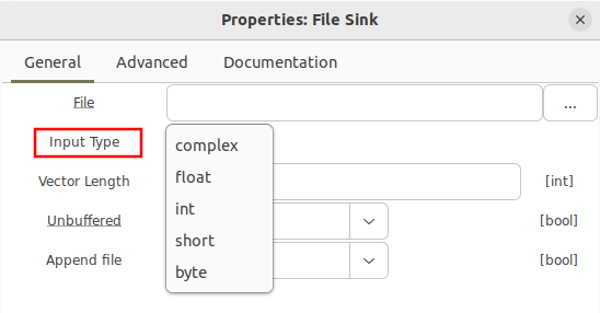
Opening the block's properties, other formats can be selected from the drop down menu:
Another common type is float, represented by orange, which writes real samples as 32-bit floats.
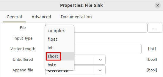
Data may also be written as 16-bit integers using the short type represented by yellow. Both real and complex samples may be written with this type, which will be discussed later in this tutorial.
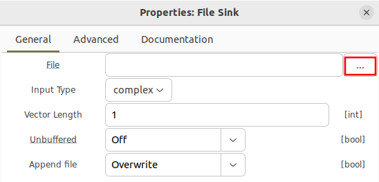
The File Sink also has a File parameter which needs to be defined. Click on the three dots:
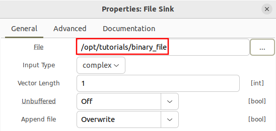
On Ubuntu a window will appear which will allows navigation to different directories so the file can be saved. The file can be saved anywhere, including the home directory although for this example it is saved in /opt/tutorials and the output filename is binary_file.
The path can also be entered directly as a text string:
Note that by default a file sink uses the Overwrite function, meaning each time the flowgraph is run the binary file in that location will be replaced by all of the new samples. The Append function is described later in this tutorial.
Filenames: Data Format
When writing binary files it is important to make a record of important metadata such as the sampling rate, binary format and others. This can be done with more complicated blocks such as File Meta Sink or SigMF Sink, however in the following examples the metadata will be stored in the filename of the binary file.
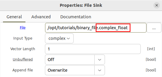
It is good practice to have readable file names when saving samples to file. The first is to include the type of data in the filename. For example, a binary file of complex samples represented by 32-bit floats could be given the file extension .complex_float. This can be added to the File Sink properties:
The following are suggested file extensions:
- Complex samples represented by 32-bit floats: .complex_float
- Complex samples represented by 16-bit integers: .complex_int
- Real samples represented by 32-bit floats: .real_float
- Real samples represented by 16-bit integers: .real_int
Filenames: Recording Sample Rate
It is also good practice to record the sampling rate in the filename. This can be automated through the use of a variable.
First change the samp_rate variable to 100 kHz (10*10**3):
Add a new Variable block to the flowgraph and convert the samp_rate number into a string. The number is converted into an integer before string conversion to make the text easier to display in the filename:
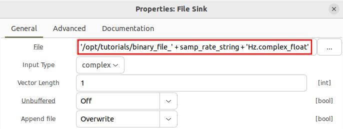
The sample rate is included in the filename through string concatenation. Note that using the file navigator button to the right of the filename will overwrite any variable-based filenames you have entered.
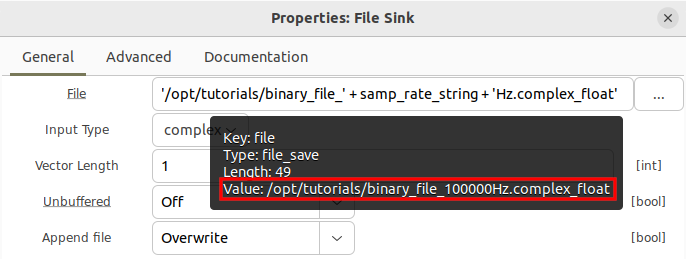
Since the samp_rate variable was changed to 100,000 the file will be saved to: /opt/tutorials/binary_file_100000Hz.complex_float
Holding the cursor over the File property will bring up summary information, including the string with all values substituted, which can be used to verify that the string has been formatted correctly before running the flowgraph:
Filenames: Using a Variable
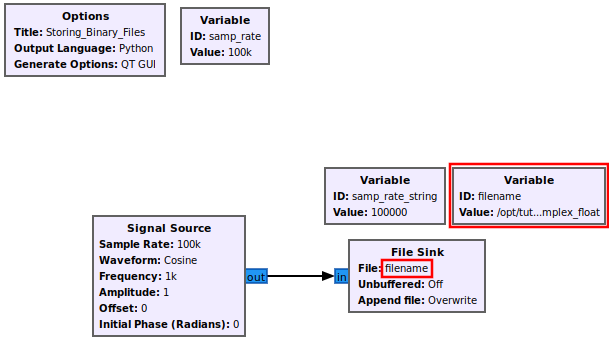
The File field can be simplified by using a variable. Copy the text into a new variable block and name it filename:
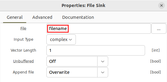
Now update the File Sink block and replace the long string with filename:
The File Sink will now use the filename variable which can be changed and modified through other variables, and those changes will be incorporated when the flowgraph starts and the binary file is written.
Filenames: Timestamping
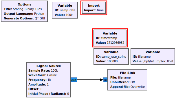
It is also useful to timestamp binary files at the time they are written. Add the Import block to the flowgraph and import the time library:
Now create a new variable named timestamp:
The int() is done to only take the integer part of the timestamp so it disregards any fractional seconds, and the str() converts the integer into a string so it can be concatenated to the filename. The timestamp is done in seconds since January 1, 1970 [1].
Notice that the timestamp in the flowgraph above is evaluated at the time the properties block was closed, however the function call will determine the proper timestamp at run time.
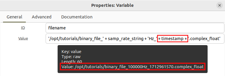
Now update the filename variable to include the timestamp through string concatenation:
Opening the Python flowgraph shows that the timestamp will be evaluated at run-time and therefore will have an accurate record of when the file was written:
Navigate to the directory the files are stored in, which in this case is /opt/tutorials. The different filename formats can be seen for each of the examples:
Writing Complex 32-bit Floats
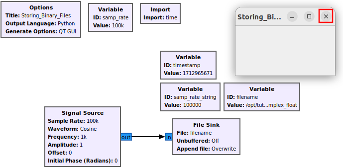
Add a Signal Source block, connect it to the File Sink and run the flowgraph for a second or two and then stop the flowgraph.
The flowgraph will now start running and will pop up a QT GUI window, but it is not populated because there are no plot blocks in the flowgraph. Data is continually being written to the file as the flowgraph is running. Close the QT GUI window to stop the flowgraph:
Navigate to the directory where the file is stored. For this example, the file was saved to /opt/tutorials.
On a Linux-based operating system the file size can be measured with the following terminal command:
$ ls -lah
The following represents the output of the command:
user@hostname:/opt/tutorials$ ls -lah
total 3.1G
drwxr-xr-x 2 user user 4.0K Date 12:41 .
drwxr-xr-x 5 root root 4.0K Date  18:15 ..
-rw-rw-r-- 1 user user 3.1G Date 12:48 binary_file_100000Hz_1712960752.complex_float
The last line shows that the file is 3.1 GB! Your exact file size may be different based on the speed of your CPU and how long you run your flowgraph.
Digitized sample files grow quickly so be sure avoid filling up the memory storage or problems can arise. From the 3.1 GB, we can work backwards to determine approximately how many complex samples are in the file. Each complex sample writes the I as a 32-bit float and the Q as a 32-bit float, therefore each complex sample is 64 bits or 8 bytes. The ratio computing the ratio of file size to the size of each sample shows there are roughly 3.1 GB / 8 bytes = 387,500 complex samples written in the file.
Writing Real 32-bit Floats
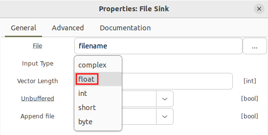
A similar process is used to write real samples as 32-bit floats. First change the file extension for the filename variable to real_float:
The data type for the File Sink is changed to float:
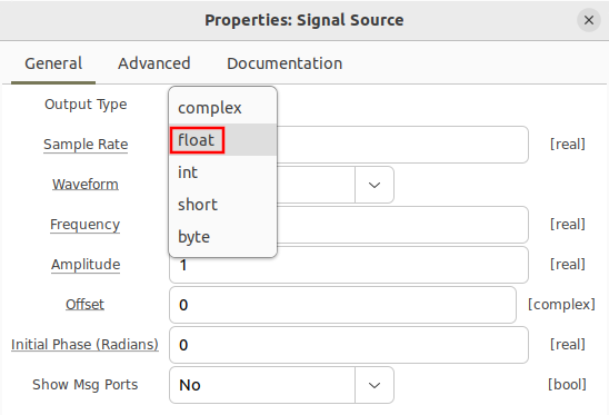
The Signal Source block is also changed to produce real floats:
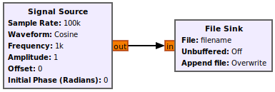
The flowgraph should now look like the following:
Running the flowgraph will write a brand new file consisting of real samples encoded as 32-bit floats to the specified location.
Writing Complex 16-bit Integers
Writing complex samples as 16-bit integers takes a couple extra steps. First change filename extension to complex_int:
Then change the Signal Source block to complex type. Then change the data type of the file sink to short:
Then add the Complex to IShort Block and connect it accordingly.
The IShort denotes the data type as interleaved 16-bit integers. Notice there is a scale factor parameter in the Complex to IShort block. 32-bit floating point numbers have a wider range of values they can represent than 16-bit integers, therefore the scale factor is needed to help perform the conversion. In this example, the Signal Source block generates a waveform with values between -1 and 1. However, 16-bit integers can only represent integer values from (-2^15)-1 to (2^15). Therefore the complex values need to be scaled to make full use of the dynamic range of the 16-bits. This is accomplished by setting the scale factor to 2^15:
The flowgraph should now look like the following:
Running the flowgraph now writes the complex samples as interleaved I and Q, with I being written as a 16-bit integer and Q being written as a 16-bit integer.
Writing Real 16-bit Integers
Writing real samples as 16-bit integers is similar to the process of writing complex samples as 16-bit integers. The File Sink also uses the short type, and add the Float to Short block. Note that the data type is Short and not IShort, because the real samples are not interleaved like the complex samples.
First change the file extension to real_int:
Connect the following flowgraph:
The scale factor needs to be updated to 2^15:
The updated value is reflected in the flowgraph:
Running the flowgraph now saves the real samples as 16-bit integers to file.
File Append
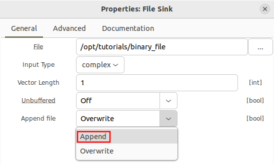
The File Sink block has an option to Append samples to the saved binary file. This means the existing binary file will not be overwritten, only added onto at the end of the file. This is selected by the Append option from the Append File option.
Reading Binary Files
This tutorial describes how to read binary files using the File Source block along side how to diagnose potential errors.
Please review the Writing Binary Files tutorial before continuing. A series of binary files were created with different formats that will be needed for this tutorial:
File Source Block
The File Source block reads from a binary file and then sends the samples to the output port. Drag the File Source block into a flowgraph. The block by default uses the complex data type (32-bit floats), represented by the blue output port:
Double clicking the File Source block brings up the properties and the ability to select different data types.
A binary file of real floating point data requires the float data type to be selected, which outputs real floating point samples, denoted by an orange output port.
A binary file of 16-bit signed integers requires the short data type to be selected, which outputs 16-bit integers of either real or interleaved I and Q samples (more on this later in the tutorial), denoted by a yellow output port.
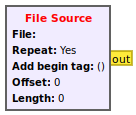
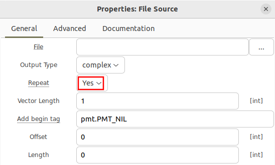
Also note that the File Source has the Repeat field enabled as Yes, which will continually and repeatedly play back the same file. Once the last sample is received in the file it skips back to the first sample in the file and continues cycling through the file.
Reading Complex Float
Add a File Source block, open the properties and begin by selecting the complex type.
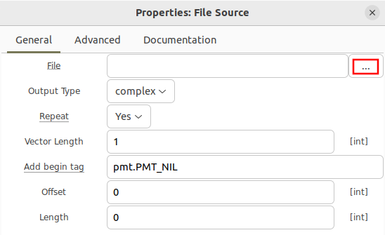
Click the three dots to the right side of the File property to browse to a stored binary file.
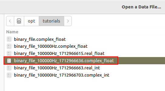
Select the file ending in .complex_float:
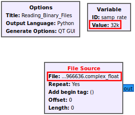
The File Source block will now populate the filename:
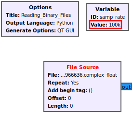
Notice that the filename is now filled in for the File Source however the samp_rate variable is incorrectly 32 kHz (32,000). The sampling rate from the filename is 100 kHz (100,000) therefore update the samp_rate variable:
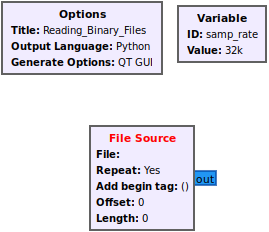
The change will be reflected in the flowgraph:
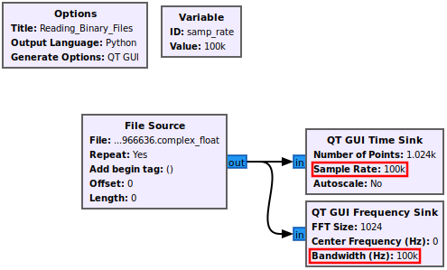
Add in the QT GUI Time Sink and QT GUI Frequency Sink and connect them accordingly. Notice how both blocks use samp_rate variable automatically:
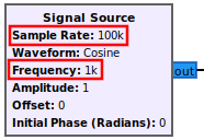
Before running the flowgraph, recall that the Writing Binary Files generated a 1 kHz complex sinusoid at a sampling rate of 100 kHz. When playing the file using the File Source the same waveform should be seen.
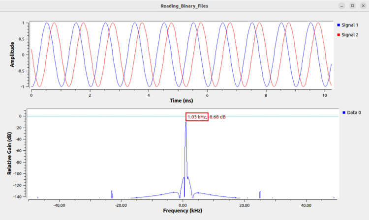
Now run the flowgraph. Notice that the time-domain plot has sinusoidal shapes on the I and Q channels, characteristic of a complex sinusoid. Also notice how the frequency plot displays a tone with a single peak, also characteristic of a complex sinusoid. Finally, notice how the peak of the frequency plot has a peak of approximately 1 kHz confirming that the binary file was read properly and the samp_rate variable was set properly.
Reading Real Float
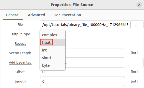
To read from a file storing real samples encoded as floating point numbers, open the File Source and change the Output Type to float:
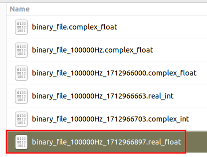
Click the three dots next to File and select the file ending in .real_float:
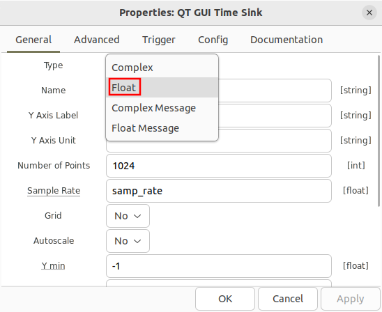
Open the QT GUI Time Sink properties and change the type to float:
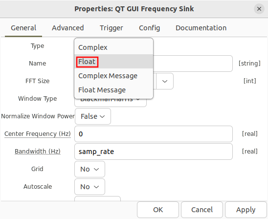
Open the QT GUI Freq Sink properties and change the type to float:
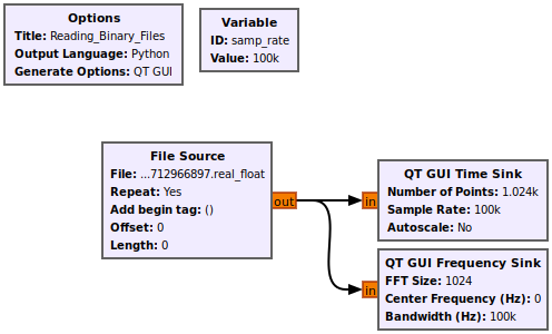
The flowgraph should now look like the following:
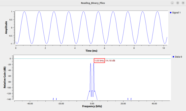
Run the flowgraph. Notice that the time-domain plot displays a single sinusoid, characteristic of a real sinusoid waveform. Also notice that the frequency domain plot displays two peaks, characteristic of a real sinusoid. Finally, notice that the peak on the right hand side, the positive frequencies, is at approximately 1 kHz, confirming that the binary file was read properly and the samp_rate variable is set properly.
Reading Real Integers
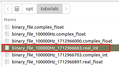
Begin by adding a File Source block. Open the properties and navigate to the file ending in .real_int:
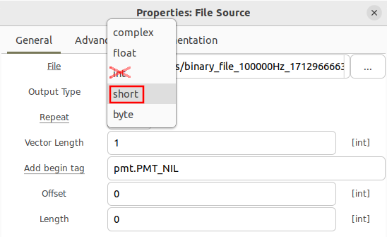
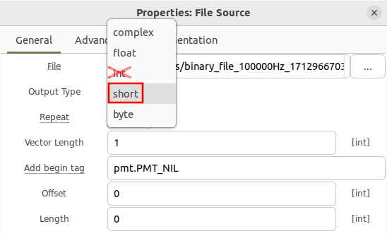
Change the Output Type property to be short. Be sure not to select int:
Add in a Short to Float block and connect it accordingly:
Notice that the scale factor here is set to 1. This will plot all of the values at full scale, which is from to , or 32,768 to +32767. Running the flowgraph with a scaling value of 1 is valid, although some flowgraphs may use a scale factor in order to normalize the data to be within -1 to +1. Open the Short to Float properties and enter a scale factor of 2^15:
The Short to Float block applies the inverse of the scale factor, meaning it will scale the output samples by or 1/32768. The flowgraph will now look like the following:
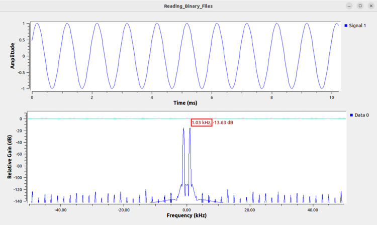
Running the flowgraph displays the file after being read as real integers. The time domain plot displays a single sinusoid which is characteristic of a real sinusoid, and the frequency domain plot displays two tones which is also characteristic of a real sinusoid. Finally, the peak at the positive frequency tone is approximately 1 kHz which confirms that the file is being read correctly.
Reading Complex Integers
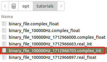
Begin by adding a File Source block. Open the properties and navigate to the file ending in .complex_int:
Open the File Source properties and select the short data type. Do not select the int type:
Drag in a IShort to Complex block and connect it accordingly. Convert the QT GUI Time Sink and QT GUI Frequency Sink blocks into the complex data type. The flowgraph should look like the following.
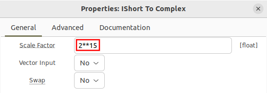
Note that the IShort to Complex block has a scale factor of 1, which would plot the data on a range of to , or -32,768 to +32,767. Running the flowgraph in this state is valid. However, some flowgraphs require normalization such that all values are within -1 and +1. To do so, open the block’s properties and use a scale factor of :
The IShort to Complex block will apply the inverse of the scale factor, or 1/32768, producing normalized samples from -1 to +1.
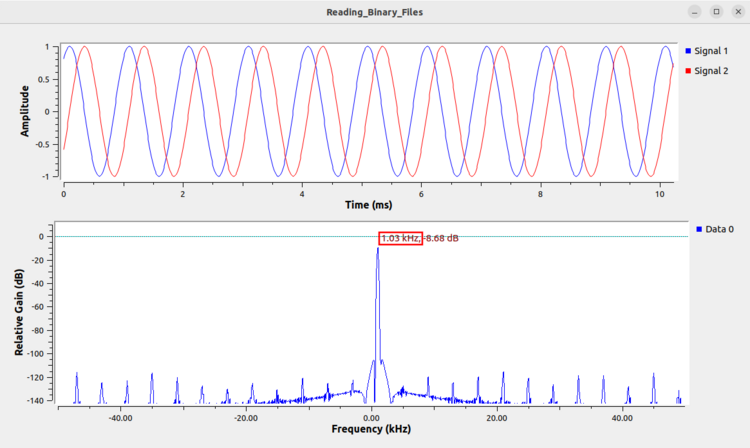
Run the flowgraph. The time domain plot displays two sinusoids, characteristic of a complex sinusoid. The frequency domain plot displays a single tone, also characteristic of a complex sinusoid. Finally, the tone is at approximate 1 kHz which confirms that the file is being read correctly.
Continuous Playback from File
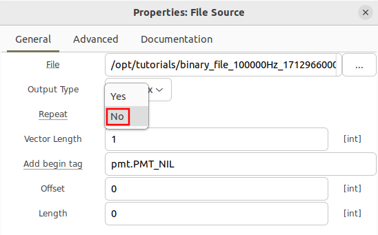
The File Source block comes with the option to repeat playback from file. When Yes is selected for repeat, the samples will be played back on loop until the flowgraph is stopped.
When No is selected for repeat, then all of the samples will be read from file and then the flowgraph will stop running once the last sample is read and then processed through the flowgraph.
Diagnosing Errors: Wrong Type and Format
In order to properly read a binary file both the type (real or complex) and format (integer or floating point) need to be known. If given a file and the type or format is unknown, it is best to check all possible combinations and to see which is the most reasonable. Endianness (described in the next section) is another potential problem when reading binary files.
The following are examples of a file being read improperly. Warning: different recordings will present different type and format errors differently, the images presented here are not exhaustive and are only a couple of examples to help build intuition to diagnose these kinds of errors.
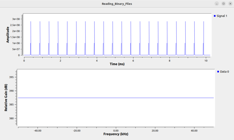
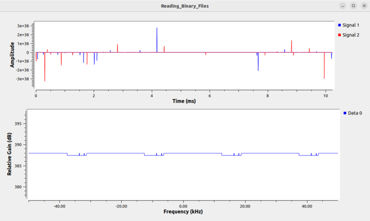
The following image is an example of a real integer being read as real floats. Note how large the values are in the time domain: on the order of ! Values that are abnormally small or abnormally large clearly indicate the file is not being read correctly.
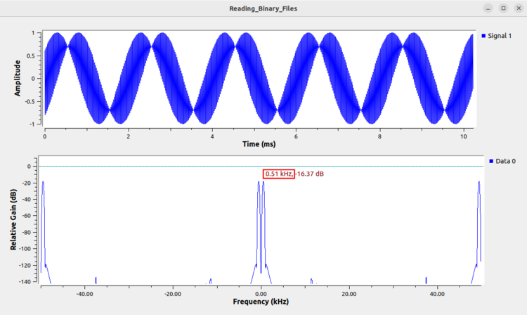
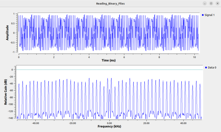
The following image is an example of complex floats being read as real floats. This kind of error can be deceptive because both the time domain and frequency domain are reasonable. The time domain has a semi-sinusoidal effect and the frequency domain has a series of peaks. Without knowing the underlying data, it could be reasonable to assume this file is being read correctly. However, it is important to try the different combinations of type and format, and reading the file as complex floats should more clearly reveal the true nature of the file.
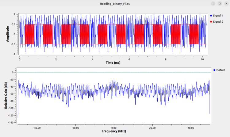
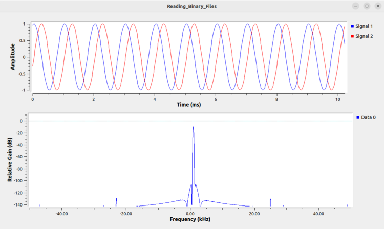
The following image shows the result when a complex floats are read as complex integers. Note that the imaginary portion of the time domain in the red represents a very strange shape which is suggestive that the file is being read incorrectly. Similarly, the frequency domain plot does not display a clearly intelligible signal.
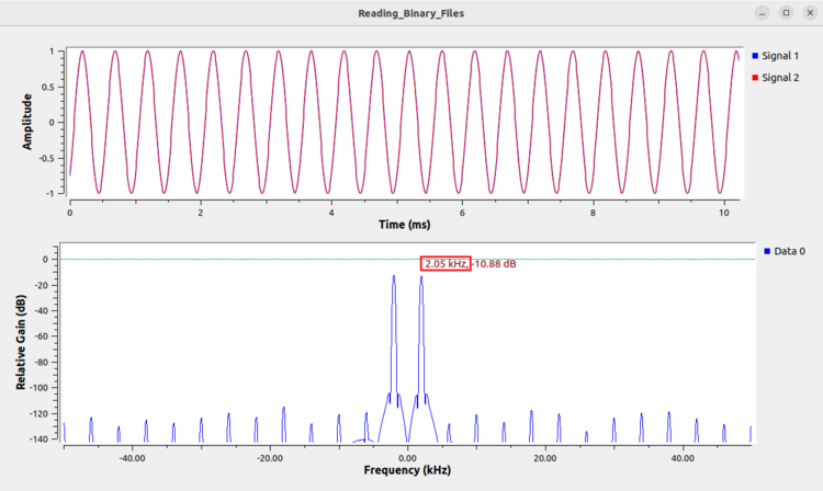
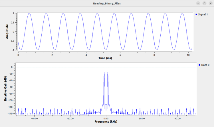
The following image is a binary file of real integers being read as complex integers. This one is tricky because at first glance it appears to be tricky, but for a complex sinusoid the real and imaginary data should be pi/2 radians out of phase with one another. Also note that the highlighted frequency is 2 kHz, and not 1 kHz as it should be, another indicator that the file was not read correctly. This is an example of why it it is important to try the different combinations of type and format, such that reading the file as complex integers should allow the user to recognize the signal is being read correctly.
Diagnosing Errors: Endianness
Endianness describes the ordering of the bits,from most significant bit (MSB) to least significant bit (LSB). Different processing architectures use different endianness and that is another factor effecting how binary files are interpreted. Endianness is only a potential problem when dealing with files from different processing systems, and therefore not an issue when performing playback from a capture taken from the same native system.
The following image is an example of a complex float file being read using the incorrect endianness:
The values being abnormally large (10^38) is a clear indicator that the file is being read incorrectly. Add the Endian Swap block to the flowgraph at the output of the File Source:
Running the flowgraph now displays the correct result:
The following image is an example of real integers being read with the incorrect endianness:
This error can be correct by using the Endian Swap block and selecting the short data type and connecting it in the flowgraph after the File Source:
Running the updated flowgraph now displays the correct result:
The next tutorial, RTL-SDR FM Receiver, describes how to build a broadcast FM receiver using an RTL-SDR receiver.

