Creating Your First Block

Beginner Tutorials Introducing GNU Radio What is GNU Radio? Installing GNU Radio Your First Flowgraph Flowgraph Fundamentals Python Variables in GRC Variables in Flowgraphs Runtime Updating Variables Signal Data Types Converting Data Types Packing Bits Streams and Vectors Hier Blocks and Parameters Creating and Modifying Python Blocks Creating Your First Block Python Block With Vectors Python Block Message Passing Python Block Tags DSP Blocks Low Pass Filter Example Designing Filter Taps Sample Rate Change Frequency Shifting Reading and Writing Binary Files SDR Hardware RTL-SDR FM Receiver B200-B205mini FM Receiver

This tutorial shows how to create a signal processing block with the Embedded Python Block. The example block will either add or multiply the two inputs based on a parameter.

This tutorial uses the Embedded Python Block which can only be used in the flowgraph it was created in. The tutorial Creating Python OOT with gr-modtool demonstrates how to create a custom Python block as an out-of-tree (OOT) module which can be installed and used in any flowgraph.

The previous tutorial, Hier Blocks and Parameters, describes how to create a hierarchical block and how to use parameters. The next tutorial, Python Block with Vectors, demonstrates how to write an Embedded Python Block with vector inputs and outputs.

Opening Code Editor

The Embedded Python Block is a tool to quickly prototype a block within a flowgraph. Search for the Python Block and add it to the workspace:

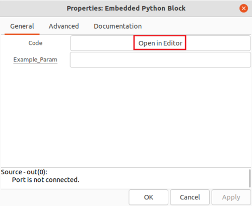
Double-click the block to edit the properties. The Embedded Python Block has two properties,

1. Code, a click-box which contains a link to the Python code for the block and
2. Example_Param, an input parameter to the block.

Click on Open in Editor to edit the Python code:

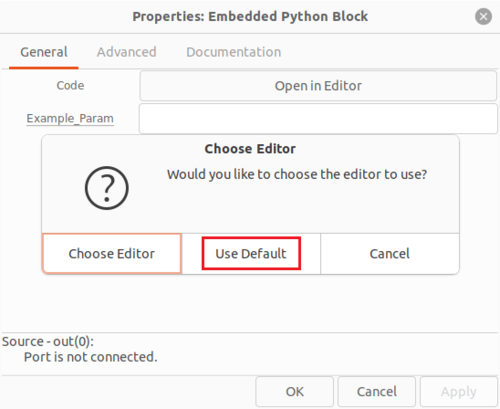
A prompt is displayed with a choice of which text editor to use to write the Python code. Click Use Default:

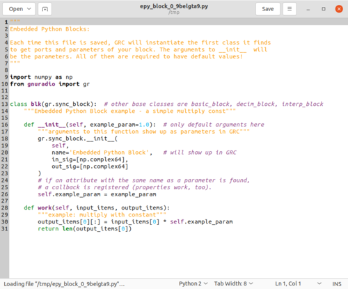
An editor window displays the Python code for the Embedded Python Block:

Components of a Python Block

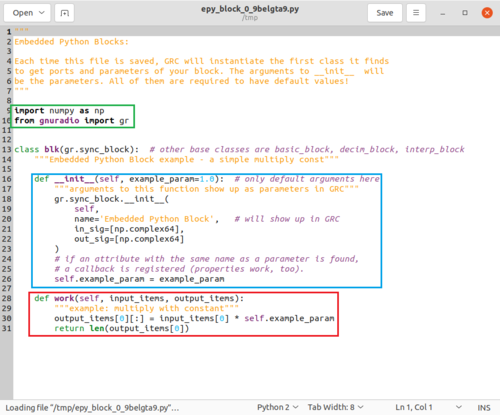
There are three important sections in the Python block code:

1. import statements in green
2. __init__ function in blue
3. work function in red

The import statement includes the NumPy and GNU Radio libraries.

The __init__ statement:

1. Accepts the example_param parameter with a default argument of 1.0
2. Declares the block to have a np.complex64 input and output, which is the GNU Radio Complex Float 32 data type
3. Stores the self.example_param variable from the input parameter

The work function:

1. Has the input input_items and output output_items parameters
2. Applies a mathematical operation to input_items and stores the result in output_items
3. Returns the number of samples produced

Changing Parameter Name

The code is modified to add the custom behavior.

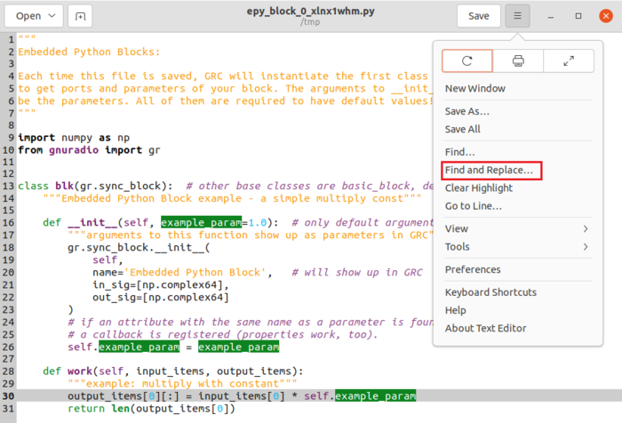
The first step is to rename example_param to additionFlag to be more descriptive. From the editor menu select Find and Replace:

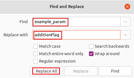
Enter:

• Find > example_param
• Replace with > additionFlag
• Click Replace All

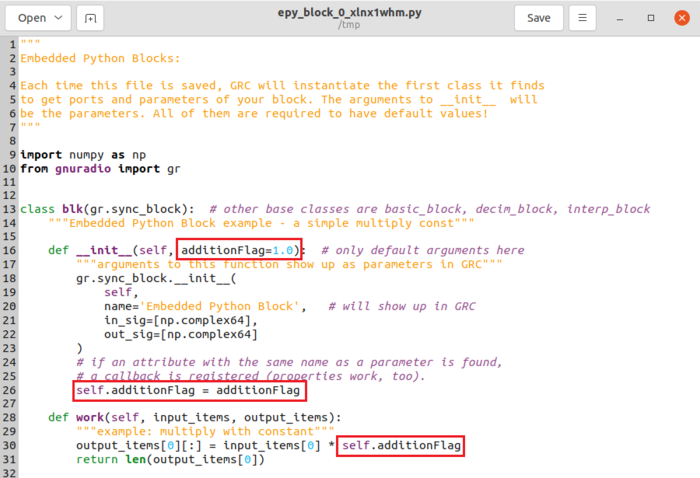
The parameter is changed. The Python code is updated:

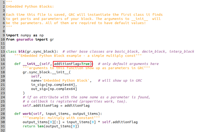
Change the default value to be True:

Save the file:

Return back to the GRC window.

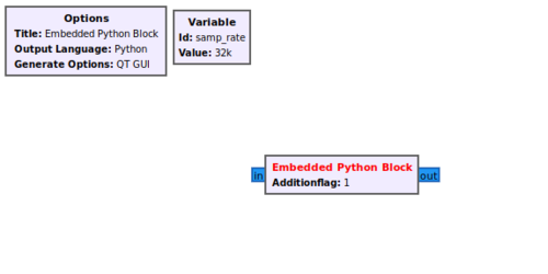
The Embedded Python Block displays the Additionflag parameter instead of example_param:

Editing Block Inputs

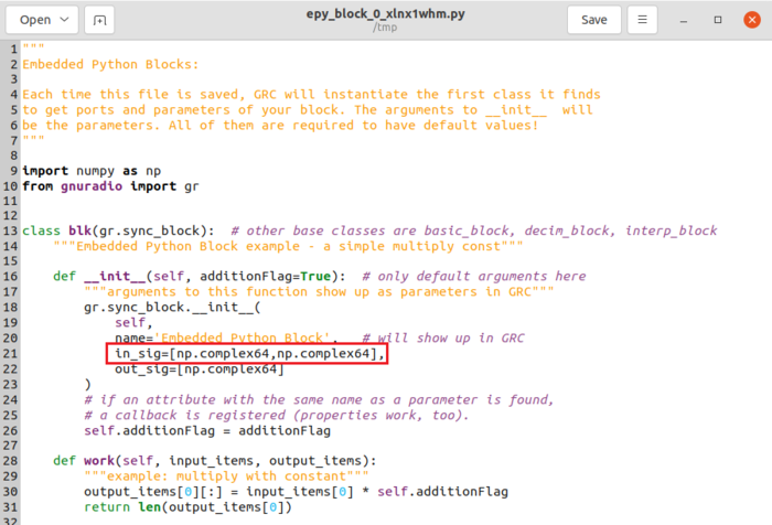
The default block has a single input and a single output, however we need two inputs for the block. To add an input, add a second np.complex64 to the in_sig list:

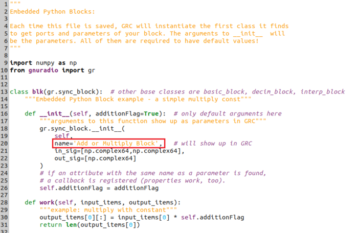
Change the block name to Add or Multiply Block:

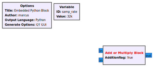
Save the file. GRC displays the block with a second input and the block name is updated:

Editing Work Function

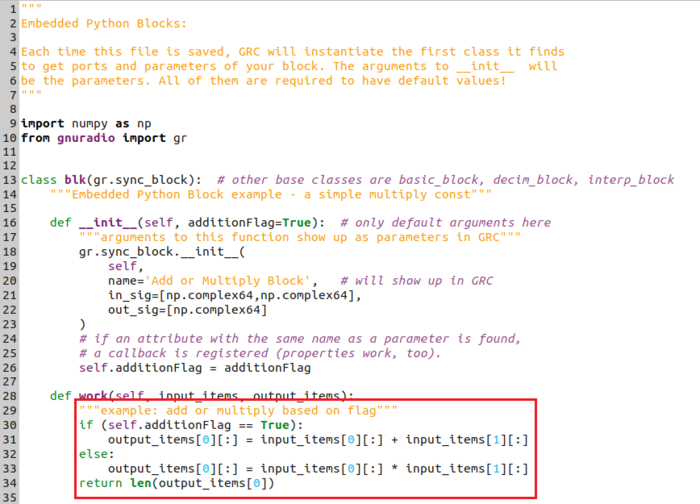
Now that the variable name has been changed the work function needs to be re-written to provide the desired functionality.

The pseudo code for the Python block is:

if (additionFlag is True)
    then add the two inputs
else
    then multiply the two inputs

Modify the work function so it has the following code:

Remember to indent with multiples of 4 spaces (4, 8, 12, etc.) when starting new lines in Python!

Save the the code.

Connecting the Flowgraph

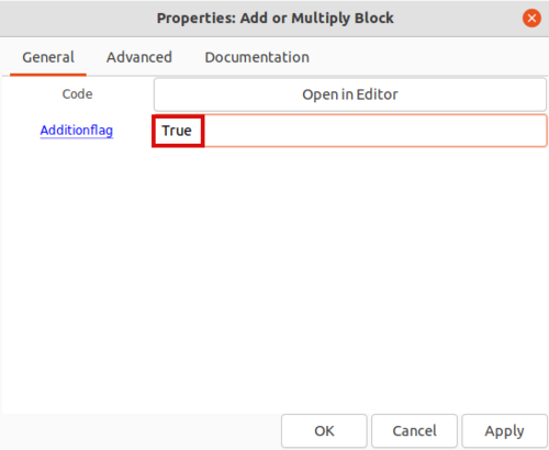
Return to GRC. Double-click the Add or Multiply Block. Enter True for the Additionflag property:

Click OK to save.

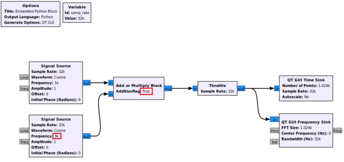
Drag and drop two Signal Source blocks, a Throttle block, a QT GUI Time Sink and a QT GUI Frequency Sink block into the GRC workspace and connect them according to the following flowgraph. Set the frequency of the second Signal Source to 3000:

Running the Flowgraph

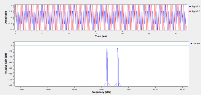
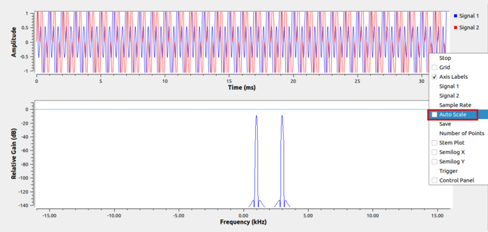
Selecting True in the Add or Multiply Block will perform the addition of the two Signal Sources. Running the flowgraph gives the following two plots:

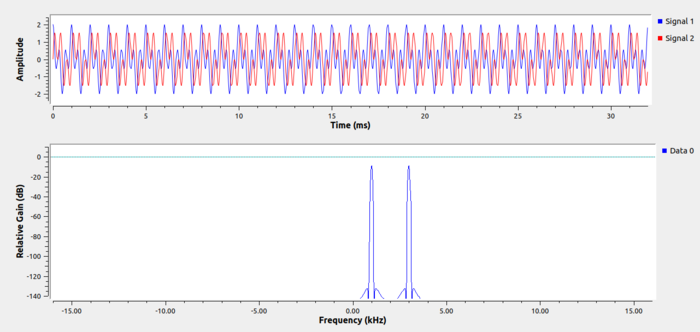
The plots show the summation of the two sinusoids, one at a frequency of 1,000 and another at 3,000. The y-axis in the QT GUI Time Sink plot is partially cutting off the amplitude of the sinusoids. Click the scroll-wheel button to bring up the display menu and select Auto Scale:

The full amplitude of the two sinusoids can then be seen:

Enter False for the Additionflag property:

Click OK to save.

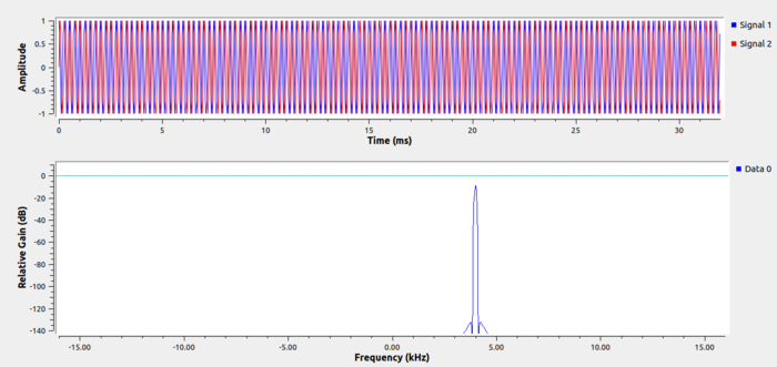
By definition, the multiplication of two complex sinusoids produces a sinusoid at the summation of the two frequencies. Therefore, the multiplication of the Signal Source of frequency 1,000 and frequency 3,000 will be a complex sinusoid of frequency 4,000. This complex sinusoid is seen when running the flowgraph:

The next tutorial, Python Block With Vectors describes how the Python Embedded Block can be modified to accept vector inputs and outputs, and how the input_items vector indexing is different between vectors and streams.